Model fitting and inference for infectious disease dynamics

What we did, the bigger picture, and where to go next

What we did

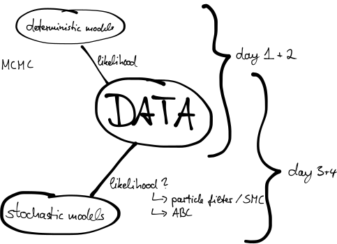
3.5 days

Monday: priors, likelihoods, posteriors, and MCMC to sample them
Tuesday: convergence diagnostics, posterior predictive checks, and the stochastic SEITL model that broke the likelihood
Wednesday: the particle filter to estimate that likelihood, pMCMC to sample with the estimate, and the observation model
Thursday: ABC, and likelihood-free inference

What happened to the likelihood

Monday. A deterministic model puts all the mass of $p(x \mid \theta)$ on one trajectory, so $p(y \mid \theta) = p(y \mid x = f(\theta), \theta)$ and you evaluate it directly.

Tuesday. The stochastic model made it an integral over every trajectory, $p(y \mid \theta) = \int p(y \mid x, \theta)\, p(x \mid \theta) \,\mathrm{d}x$ , with no closed form.

Wednesday. The particle filter estimated that integral without bias, and pMCMC sampled with the estimate.

Thursday. ABC dropped it for $p\big(d(S_y,\, S_{\text{sim}(\theta)}) < \epsilon\big)$ .

The bigger picture

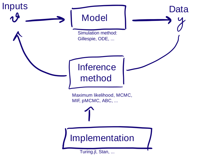
Inference in one loop

Four choices

Every fit settles four questions, whether or not you notice deciding them (Funk and King 2020). Three of them are labelled on the loop:

The model: deterministic or stochastic, and how complex
The simulation method: an ODE solver, Gillespie, or tau-leaping
The inference method: full information or summaries, Bayesian or frequentist
The software: a package, a language, or code of your own

To fit SEIT4L we picked a stochastic model, a Gillespie simulator, pMCMC, and Julia with Turing.jl.

How to choose?

The main criteria are:

A model suitable for the question at hand (model adequacy)
Being able to do the inference in the time available (computational efficiency)
Getting a correct answer (statistical accuracy)
Being able to write the model down correctly and quickly (coding efficiency)

Model adequacy

The right model comes before any inference procedure. Can it generate data like yours, for the purpose you built it for?

A deterministic model puts all the mass of $p(x \mid \theta)$ on one trajectory, so it cannot represent process noise. That matters in a small population, where stochastic fade-out is a real possibility rather than a rounding error.

Computational efficiency

Total cost is the cost of one simulation, times the number of simulations the method needs.

Cost of one simulation

The simulation method and the implementation: an ODE solver against Gillespie, compiled against interpreted.

Number of simulations

The inference method. NUTS reaches a given ESS in far fewer iterations than a random walk, and rejection ABC needs very large numbers of cheap forward simulations.

Statistical accuracy

pMCMC uses a noisy likelihood estimate and still targets the exact posterior. Run it for long enough and the Monte Carlo error falls as far as you like.

ABC does not. $\epsilon$ and the choice of $S(y)$ bound the accuracy however long you run it, so more computation sharpens an answer that stays biased.

Coding efficiency

Your time: writing, testing, debugging.

The choices interact

Software constrains method: a package implements what it implements.

The model constrains method: a model too slow to simulate rules out any procedure needing a million runs.

Probabilistic programming languages (PPLs)

In PPLs you write down the model specification, and the language takes care of the simulator and the inference.

One definition of SEIT4L, and Turing will run NUTS() on a tractable differentiable likelihood, MH() or Emcee() where there is no usable gradient, and SMC(), PG() or CSMC() where the likelihood has to be estimated from simulations. Wednesday was that: the model unchanged, the particle filter’s estimate added with @addlogprob!.

Turing.jl in Julia
Stan in R, Python or Julia
NumPyro and PyMC in Python

When things don’t work

Slow, sticky, or divergent is often the sampler, and often fixable: retune the proposal, reparameterise the model raise the particle count until the variance of the log-likelihood estimate is around one.

Biased, overconfident, or wrong is not due to the sampler.

The observation model: Poisson on overdispersed counts gives an overconfident posterior, and one outlying day dominates the fit
The priors: Uniform(1, 20) on $R_0$ says 19 is as plausible as 2
Identifiability: two parameters that trade off cannot be separated by any sampler, being a property of model and data
The model: one that cannot generate your data will not be rescued by better inference

Checking the model

Two separate modes of checking

Sampler problems: R̂, divergences, low ESS, sticky traces.

Model problems: posterior predictive checks, predictive p-values.

Both are necessary. A converged chain from a misspecified model looks exactly like a converged chain from an adequate one.

A recipe for your own model

1. Start with the question. Name the quantity you need to learn and the data that can inform it.

2. Write the generative story. Separate the epidemic process from the observation process, and decide where stochasticity belongs.

3. Simulate before fitting. Draw parameters from the prior and run the whole model. If it cannot generate plausible data, revise the model or prior now.

Fit, check, revise

4. Choose a method that fits the model and your computational budget.

5. Check the computation. Use multiple runs, traces, R̂, ESS and method-specific warnings to establish that the algorithm explored its target.

6. Check the model. Use posterior predictive checks and sensitivity analyses to ask whether the fitted model reproduces the features that matter to your question. If it does not, revise the model and go round again.

A workflow for infectious disease modelling (Abbott et al., work in progress) sets out the full version, including how to combine data sources.

Where to go next

Further topics

Variational inference: optimisation over a variational family in place of sampling, for when the answer is needed in real time
Neural posterior estimation: amortised inference with normalising flows, for a model you fit many times
Universal differential equations: a neural closure term inside the model, for the part of the mechanism you cannot write down
Beyond Turing: other samplers, automatic differentiation backends, and what sits underneath the Julia we have been using

All four are on the course site, written to be worked through on your own.

Beyond the core sessions

Across the course site, Going further and advanced sections point to extensions of the methods we taught and the literature behind them.

Nowcasting and forecasting infectious disease dynamics is our course on real-time infectious disease modelling.

Before you go

A feedback survey at bit.ly/4h086oM, also coming by email. This is the first time we have taught the material in this form, so please fill it in.
Everything here stays online and is MIT licensed. Reuse it, with attribution.
The Discussion board is for questions, and for showing what you have fitted.
Open an issue for anything wrong, unclear or broken. That helps the next cohort.