Introduction to Markov Chain Monte Carlo

Model fitting and inference for infectious disease dynamics

Recap

Recap: Bayesian inference

Last time we saw that the posterior distribution of $\theta$, given observed data, is

$$p(\theta \mid \text{data}) \propto p(\text{data} \mid \theta)\, p(\theta)$$

Our aim is to draw samples from this distribution.

Why sample?

Sampling to learn about a population

• Imagine you want to know the mean height of people in London.
• You cannot measure everyone, so you take a sample $S$.

$$m = \frac{1}{N_\text{Lon}} \sum_{i \in \text{Lon}} h_i \;\approx\; \frac{1}{N_S} \sum_{i \in S} h_i$$

We can do exactly the same thing to study a posterior distribution.

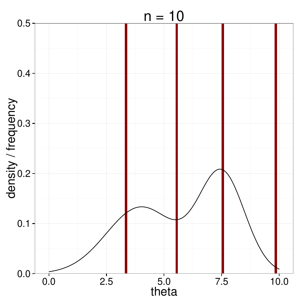
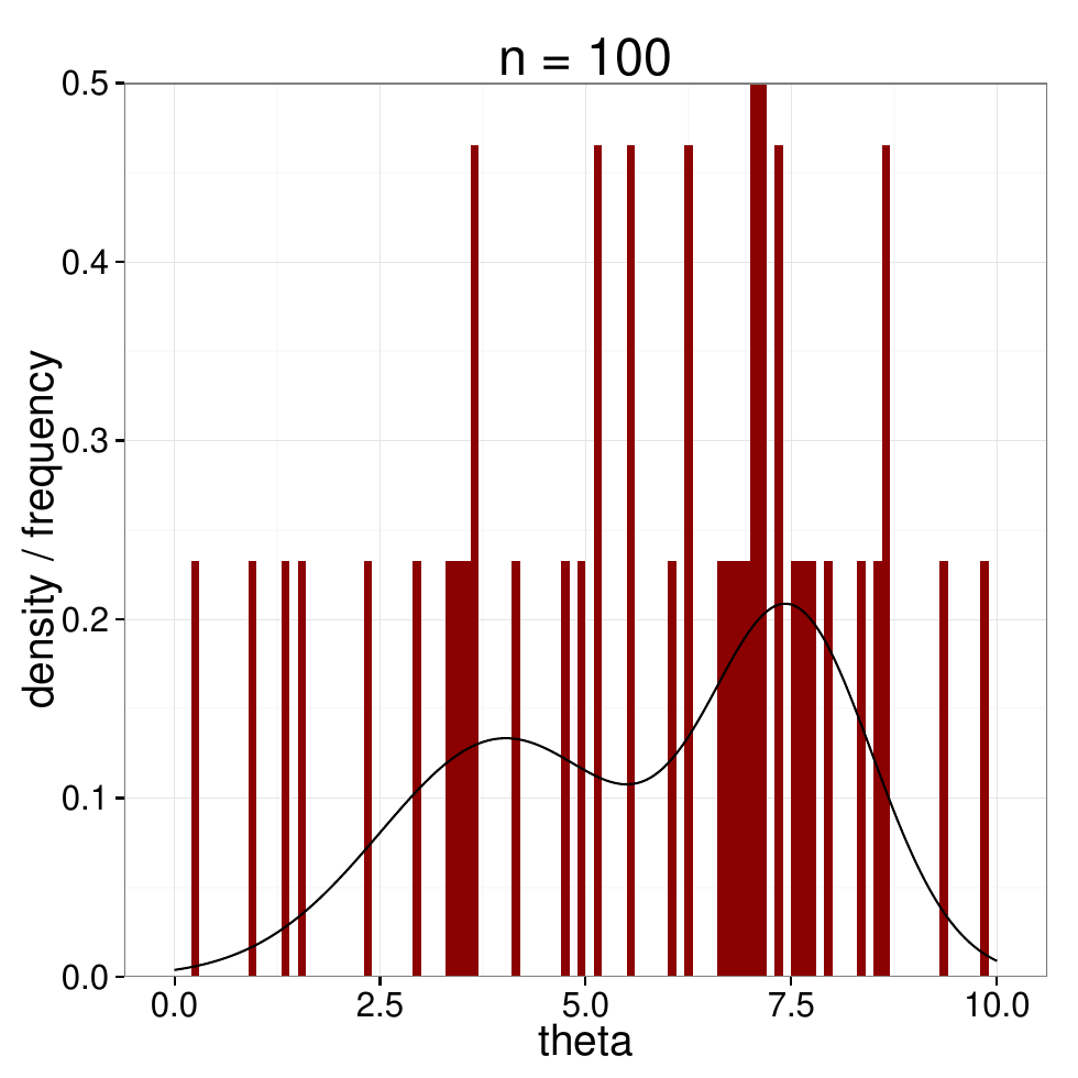
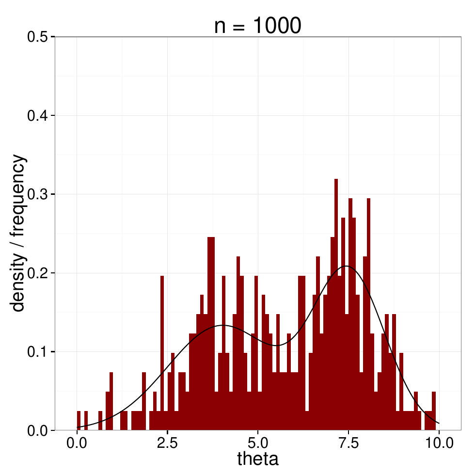
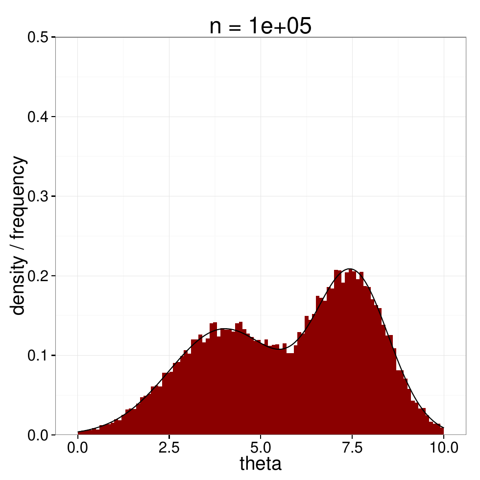
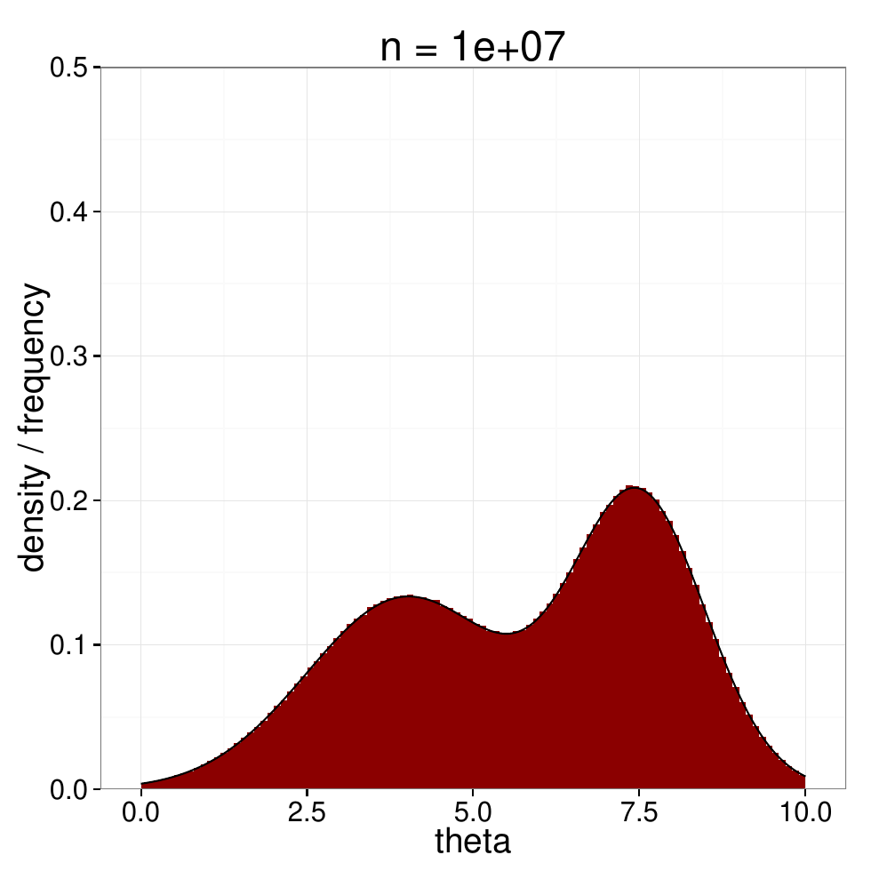
Monte Carlo sampling

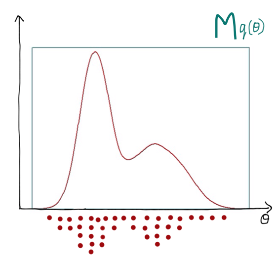
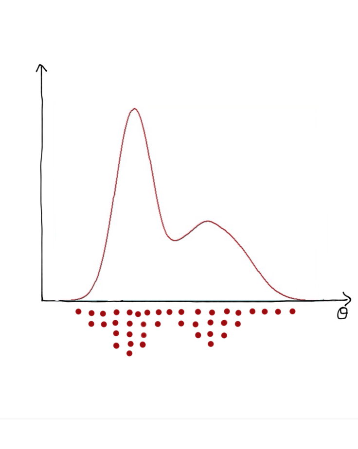
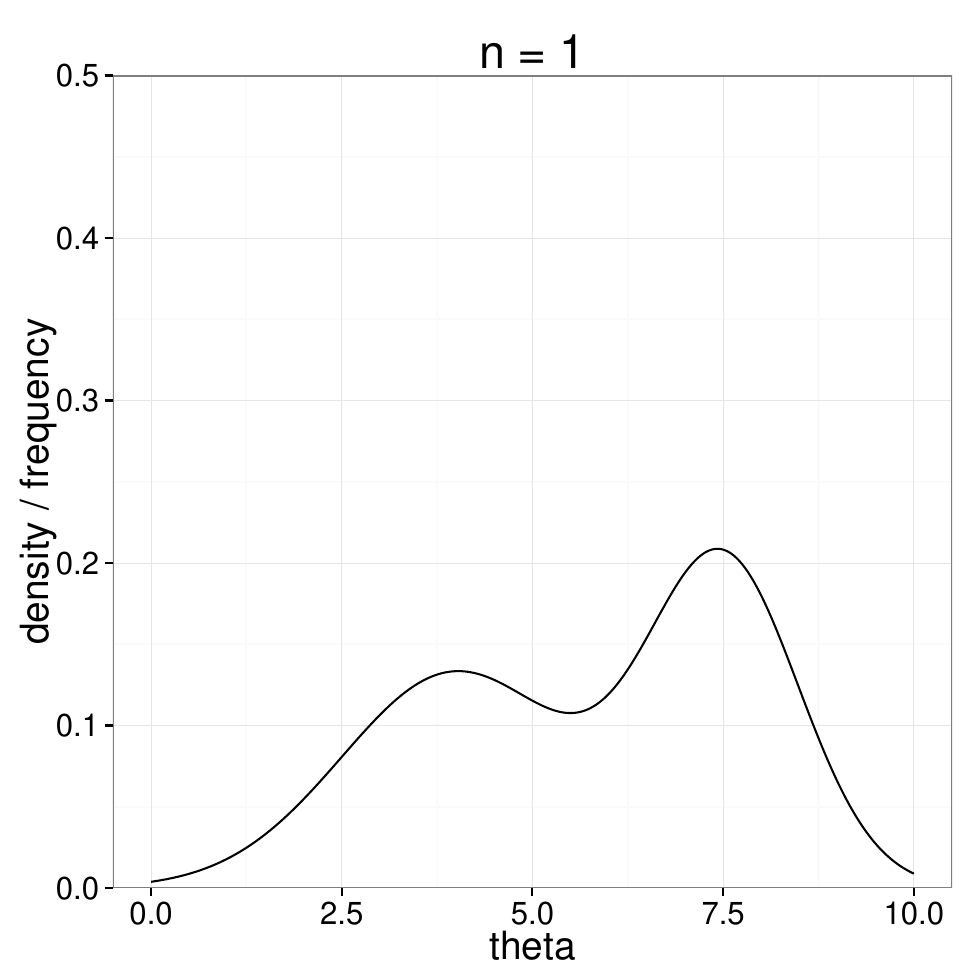
Explore a distribution by drawing from it. More samples, better picture:

Wasting time in sampling

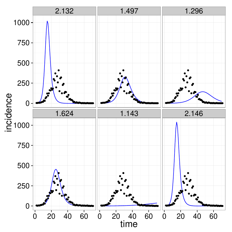
Sampling blindly from the prior spends almost all its effort on parameter values that fit the data badly. We need something that concentrates where the posterior is.

Rejection sampling

The problem

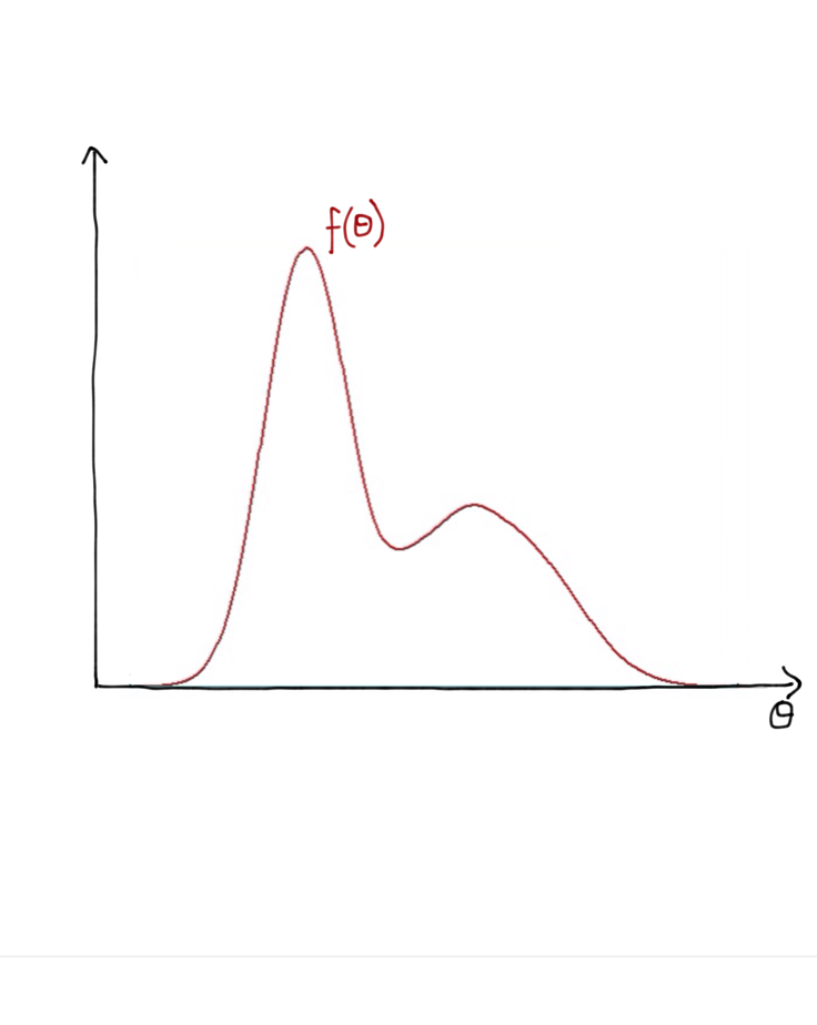
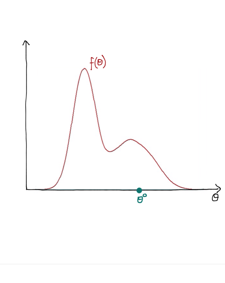
• Consider a distribution $f(\theta)$ which we can evaluate for any $\theta$
• How do we draw samples from it?

A proposal distribution

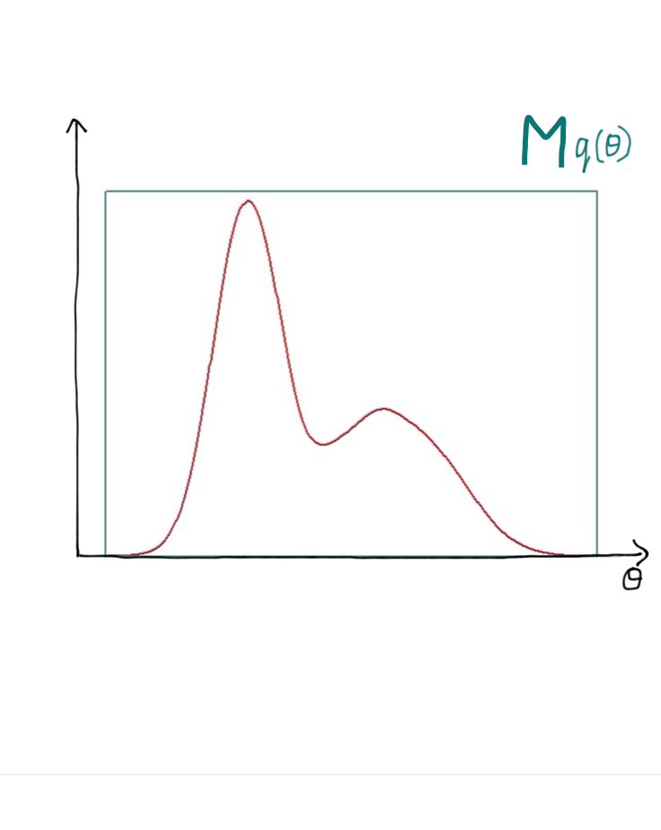
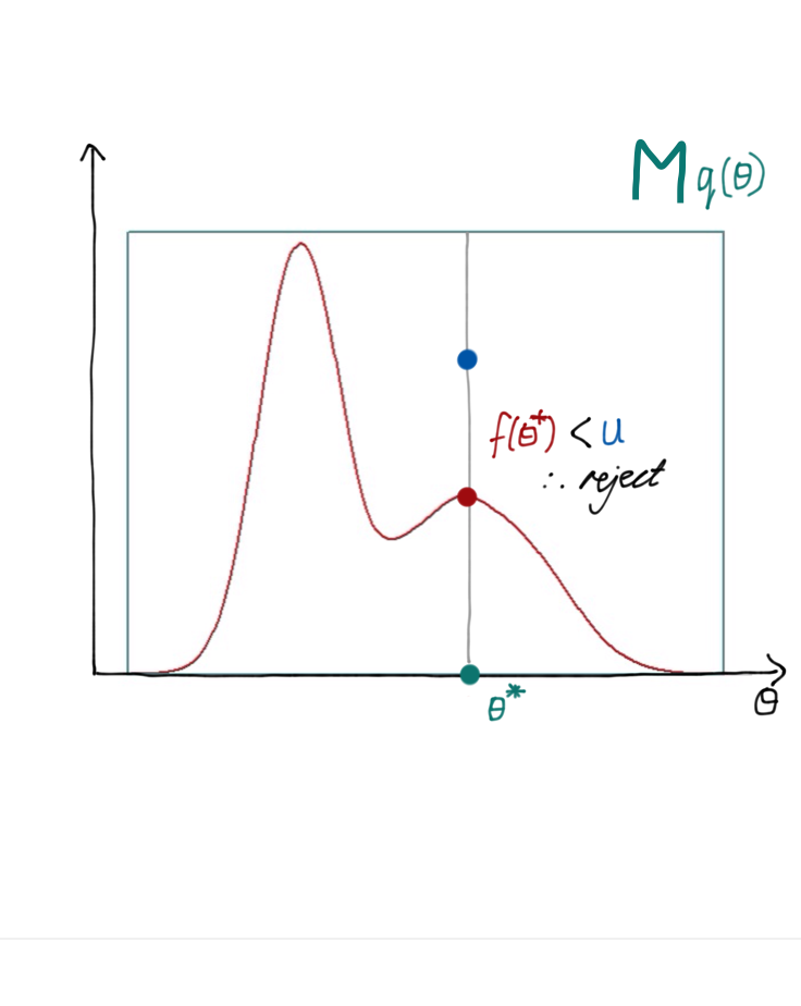
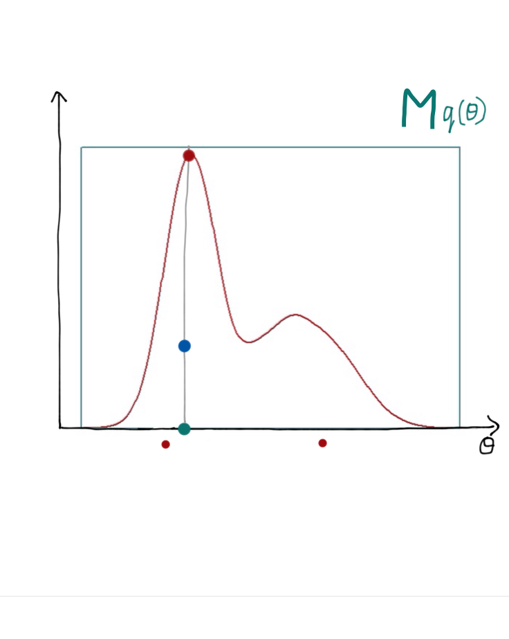
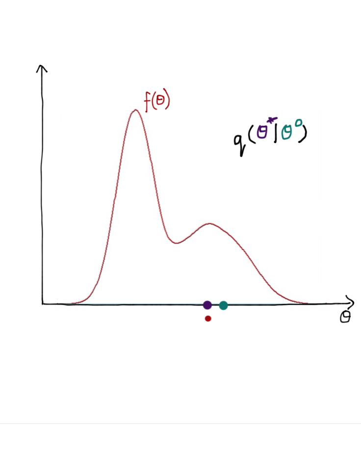
Rejection sampling uses a proposal distribution $q(\theta)$ which

• is simple to evaluate
• is easy to sample from
• admits some $M > 1$ with $f(\theta) < M q(\theta)$ for all $\theta$

The algorithm

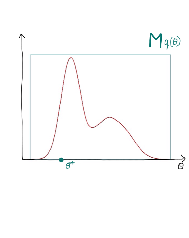
1. Sample $\theta^*$ from $q(\theta)$
2. Draw $u \sim \text{Uniform}[0,\, M q(\theta^*)]$
3. Evaluate $f(\theta^*)$
4. If $f(\theta^*) > u$ accept, else reject
5. Repeat steps 1–4

Building up a sample

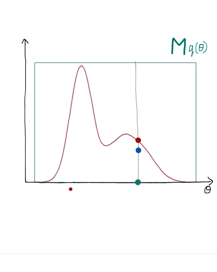
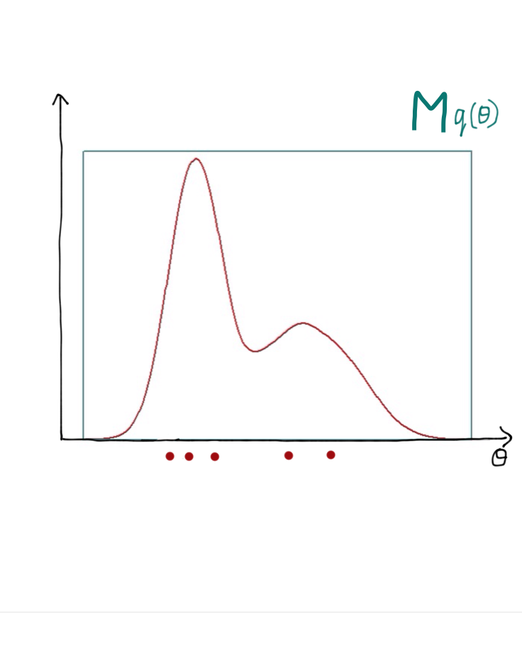
1. Sample $\theta^*$ from $q(\theta)$
2. Draw $u \sim \text{Uniform}[0,\, M q(\theta^*)]$
3. Evaluate $f(\theta^*)$
4. If $f(\theta^*) > u$ accept, else reject
5. Repeat steps 1–4

Accepted points build up a sample from $f(\theta)$.

When rejection sampling struggles

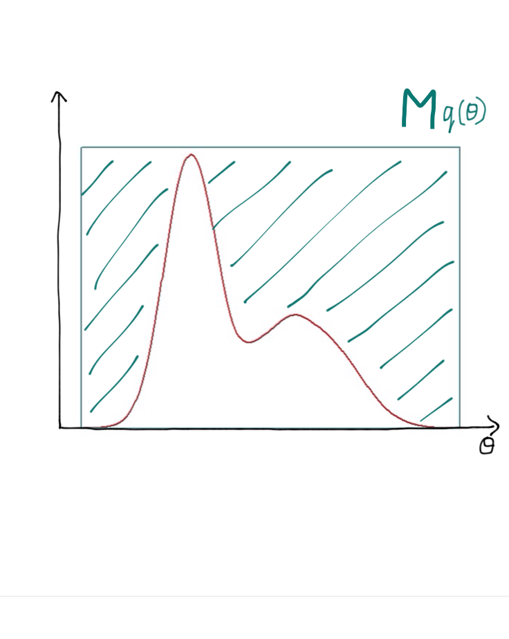
• Works best when $q(\theta) \approx f(\theta)$, i.e. $M \gtrapprox 1$
• The acceptance rate is $1/M$
• Requiring $f(\theta) < M q(\theta)$ everywhere can push the rejection rate very high
• Worse still in high dimensions

Walking towards the target

Markov chain Monte Carlo

• In Markov chain Monte Carlo (MCMC) we do not need one proposal density $q(\theta)$ that bounds $f(\theta)$ everywhere.

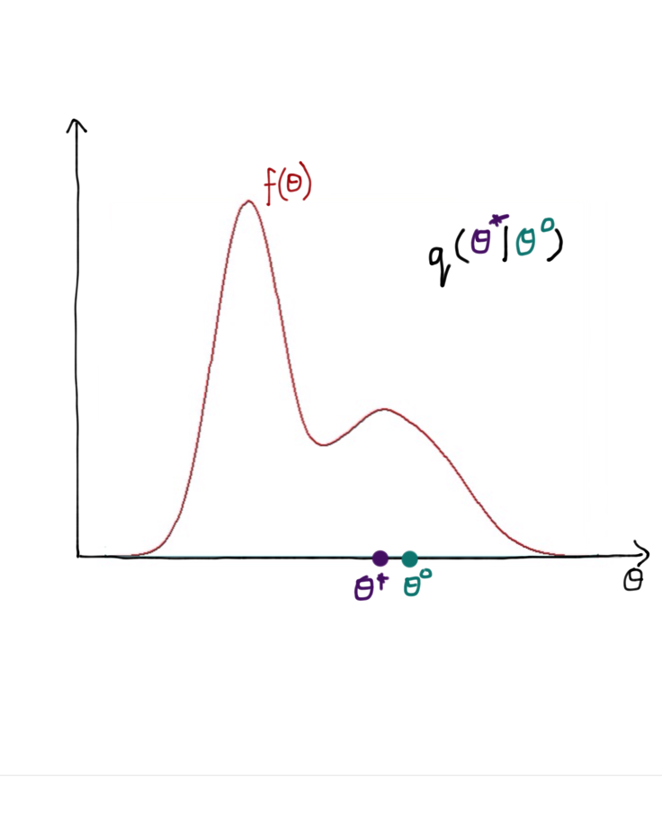
• Instead we build a chain of samples, where each proposed $\theta^*$ depends on the previous one: the proposal density takes the form $q(\theta^* \mid \theta)$.

• A commonly used MCMC algorithm is Metropolis-Hastings.

• Its acceptance rate is carefully derived to ensure unbiased samples.

Metropolis-Hastings

1. Initialise $\theta^{0}$, set $\theta = \theta^{0}$
2. Sample $\theta^* \sim q(\theta^* \mid \theta)$
3. Compute the acceptance probability $r$
4. Draw $u \sim \text{Uniform}[0,1]$
5. Set the new sample to $$\theta^{(s+1)} = \begin{cases} \theta^*, & u < r\\ \theta^{(s)}, & u \geqslant r\end{cases}$$
6. Repeat steps 2–5

The acceptance probability

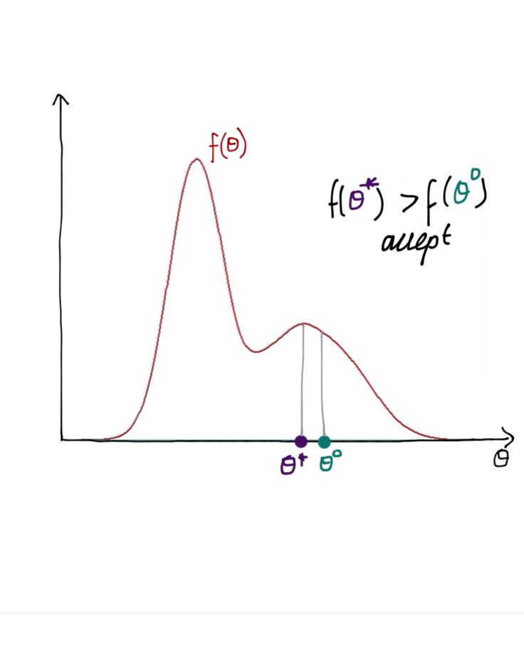
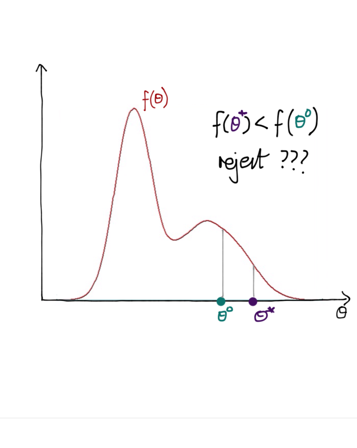
If $q(\theta^* \mid \theta)$ is symmetric, then

$$r = \min\left(1, \frac{f(\theta^*)}{f(\theta)}\right)$$

• Always move to $\theta^*$ if it is more probable than $\theta$

• May move even if $\theta^*$ is less probable

If $q(\theta^* \mid \theta)$ is asymmetric, then

$$r = \min\left(1, \frac{f(\theta^*)\,q(\theta \mid \theta^*)}{f(\theta)\,q(\theta^* \mid \theta)}\right)$$

Finding a good proposal distribution

How do we choose $q(\theta^* \mid \theta)$?

Too narrow and the chain crawls; too wide and almost nothing is accepted. The proposal has to match the shape of the posterior.

With 2 parameters that is 3 numbers to pick, and with 10 it is 55.

Worse, the shape you need is the shape of the thing you have not sampled yet.

Adaptive MCMC

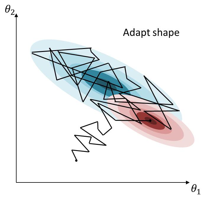
• Adaptive MCMC alters the proposal distribution while the chain is running.

• Start with a large symmetric variance and scan around to find a mode.

• Then alter the shape of the proposal to match the covariance of the accepted values.

• Eventually the proposal density should match the shape of the target density.

Adaptive MCMC: two-stage adaptation

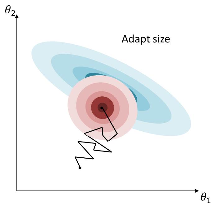
Classical adaptive Metropolis: Haario et al. (2001). Robust adaptive Metropolis (RAM), which we use in the practical: Vihola (2012).

Using gradients

Using the gradient

Metropolis-Hastings proposes a direction at random and hopes for the best.

For a model we can differentiate, and an ODE model qualifies because the solver propagates derivatives, the gradient of the log-posterior tells us which way is uphill.

Hamiltonian Monte Carlo uses it: simulate a puck rolling on the surface, with gradients pulling it towards high density and momentum carrying it a long way. The direction and length of each move now come from the posterior.

NUTS

NUTS, the No U-Turn Sampler, is HMC with the step size adapted during warmup and the trajectory length stopped when the path turns back on itself.

It usually just works, with no proposal tuning at all, and is the default to reach for. Fall back to RAM or MH for discrete parameters, or a stochastic simulator that breaks differentiation, as the particle filter will later.

Hoffman and Gelman (2014); see Betancourt (2017) for the intuition.

Your Turn

In the practical you will

• implement Metropolis-Hastings yourself for a one-dimensional target
• see what the proposal distribution does to the chain
• experience how hard tuning a proposal by hand is
• hand the same job to Turing.jl, then compare MH, RAM and NUTS

Return to the session