MCMC diagnostics

Model fitting and inference for infectious disease dynamics

Recap

Where we are

Yesterday you sampled a posterior: Metropolis-Hastings by hand, then NUTS doing the same job with gradients.

Today’s question is narrower. The sampler returned numbers. Are they samples from the posterior?

MCMC always returns something. Nothing forces it to be right.

Convergence is asymptotic

A chain has converged when its draws are distributed as the posterior, and stay that way however long you run.

That is a statement about the limit. No finite run establishes it.

So everything today is a check. Each one can show you a problem. None can show you there is not one.

Visual diagnostics

The trace plot

The parameter against iteration: where the chain has been. For NUTS, where the puck has been.

Why we like hairy caterpillars

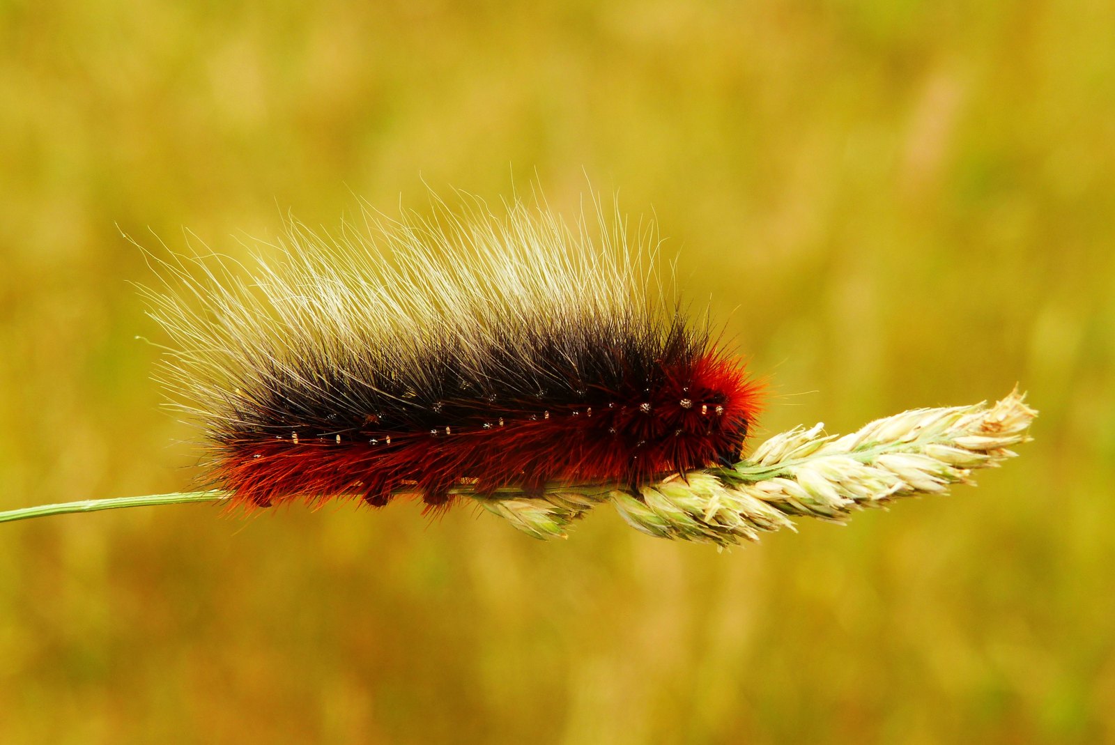
• Straight — no trend across the run
• Plump head, plump rear — the same spread at the start as at the end
• Multiple colours — several chains on top of each other

Two more plots worth making

Running mean

It should settle and stay settled.

Autocorrelation

It should decay to zero within a few tens of lags.

Still drifting, or still correlated at lag 100, and your effective sample size is a small fraction of the iterations you ran.

One chain cannot tell you it is wrong

Every plot so far looked at one chain.

A chain that settles in part of the posterior and explores it thoroughly looks healthy on all three.

It has never been anywhere else, so it cannot tell you what it missed.

Chains started apart

Chains that started apart and ended up in the same place have found the same distribution. Chains that did not have not.

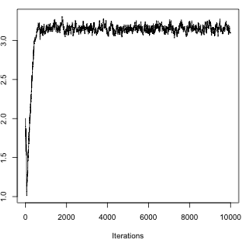
Burn-in

• We can start our MCMC chain anywhere.

• It can take a while to reach and explore the target density $f(\theta)$.

• Throw away the early samples: the burn-in phase.

• NUTS adapts during warmup and discards it for you.

How long to warm up?

NUTS adapts for min(1000, N ÷ 2) iterations by default, so 2000 draws gives 1000 of warmup. It is the first argument: NUTS(2000, 0.65).

Longer warmup buys a better step size and mass matrix. For most models the default is enough.

Less is often safe, and worth having when a model is expensive. Check R̂ and the traces are no worse before relying on it.

MCMC sample size

• In MCMC each sample depends on the one before: auto-correlation.

• Reduce auto-correlation by thinning, retaining only every $n$-th sample. Rarely needed for NUTS; useful for random-walk samplers.

• The information content of a set of MCMC samples is given by the effective sample size (ESS).

Accuracy and efficiency

How does each of these influence accuracy and efficiency?

• Burn-in
• MCMC iterations after burn-in
• Thinning
• Number of chains, with different initial conditions
• Proposal distribution
• Transforming parameters

Quantitative diagnostics

Autocorrelation as a number

$\rho_k$ is the correlation between the chain and itself $k$ steps later.

Summed, it gives the integrated autocorrelation time

$$\tau = 1 + 2\sum_{k=1}^{\infty} \rho_k$$

The 1 is each draw with itself; the 2 counts every other lag in both directions.

roughly the iterations needed for one draw’s worth of new information.

R̂: the Gelman-Rubin diagnostic

Compare the variance within each chain to the variance between chains.

$$\hat{R} = \sqrt{\frac{\hat{V}}{W}}, \qquad \hat{V} = \frac{n-1}{n}\,W + \frac{1}{n}\,B$$

$n$ draws per chain. $W$ is the mean within-chain variance. $B$ is $n$ times the variance of the chain means, so $B/n$ is that variance. $\hat{V}$ adds the two.

The same two runs as the traces earlier, now as one number.

What R̂ is telling you

Chains sitting in different places inflate $B$, and R̂ goes up with it.

Chains that agree still do not reach exactly 1, because the draws inside each chain are correlated. A chain mean varies by about $\sqrt{W\tau/n}$, so $B \approx \tau W$ and

$$\hat{R}^2 \approx 1 + \frac{\tau - 1}{n}$$

near 1 when the chain is long compared with $\tau$.

Rule of thumb: $\hat{R} < 1.1$ as a minimum, ideally $\hat{R} < 1.01$.

rhat() prints a refined version of this, so the two will not match by hand.

Rank-normalised R̂ and ESS: Vehtari et al. (2021)

Effective sample size

Correlated draws provide less information than independent ones.

$$N_{\text{eff}} = \frac{N}{1 + 2\sum_{k=1}^{K} \rho_k} = \frac{N}{\tau}$$

The sum is truncated where the estimates go to noise, in grey. Both panels are 4000 draws.

Geyer (1992)

How accurate is the reported estimate?

When reporting a posterior it matters how accurate the estimate is: how many of the digits are real, and how many would change with a different seed.

Monte Carlo standard error aims to help answer that:

$$\text{MCSE} \approx \frac{\text{posterior SD}}{\sqrt{\text{ESS}}}$$

It is in the units of the parameter, the same units as the posterior SD, so it says directly which decimal place the seed is moving.

Report $R_0 = 2.31$ with an MCSE of $0.05$ and a different seed moves the estimate by about that much. Report $R_0 = 2.3$; the second decimal needs an MCSE nearer $0.005$.

How well determined is the mean?

Note the two x-ranges. The posterior on the left is what you report. On the right, the mean of a 750-draw run over 400 repeats: that spread is the MCSE, narrower by $\sqrt{\text{ESS}}$.

So ESS is the only lever.

Common failure modes

Divergent transitions

Specific to HMC and NUTS. The sampler slides a puck along a trajectory; a divergence means that simulation became numerically unstable and the puck flew off.

This usually means the posterior has a region of sharp curvature — a funnel or a narrow ridge — where the step size that works elsewhere is far too large.

A handful of divergences may be tolerable. Many means the sampler is systematically avoiding part of the posterior, so your samples are biased, not merely noisy.

Multimodality

If the posterior has several separated modes, a chain can settle in one and never see the others.

Chains landing in different modes make R̂ large. So do chains that have simply not converged yet.

Usually a property of the model and the data, not the sampler, so the first question is which mode you believe and why.

Fixes, in the order to try them:

• a prior that rules out an implausible mode, if it is defensible on its own terms
• a mixture model, if the modes are genuinely different explanations
• a sampler designed to cross between modes

It is almost never the sampler

R̂, ESS and MCSE tell you the algorithm struggled.

Usually the cause is the model: correlated or non-identified parameters, a prior with mass where the solver fails, a badly conditioned posterior.

Reach for the model before reaching for NUTS(0.95) or a new sampler.

Your Turn

In the practical you will

• read trace, running mean and autocorrelation plots on a fitted SIR model
• watch four chains agree, and four chains fail to
• compute R̂, ESS and MCSE, and see R̂ catch the chains that disagree
• diagnose a deliberately badly specified model and try to fix it

Return to the session