Observation models

Model fitting and inference for infectious disease dynamics

Observation models

What an observation model is for

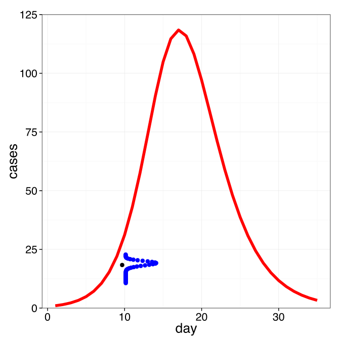
A deterministic model gives one smooth trajectory. The counts do not sit on it.

Two jobs

The distribution around the prediction is what makes a likelihood exist. The likelihood gives us a distribution around the prediction. That way the model doesn’t have to fit the data perfectly.

It is also where the observation process lives: under-reporting, and the variation of counts around what the model expects.

The choice we have been making so far

Every likelihood in this course so far has assumed

$$y_t \sim \text{Poisson}(\lambda_t)$$

where $\lambda_t$ is what the model predicts at time $t$.

That is a modelling choice. It makes a specific claim about how observation works.

What we have assumed so far

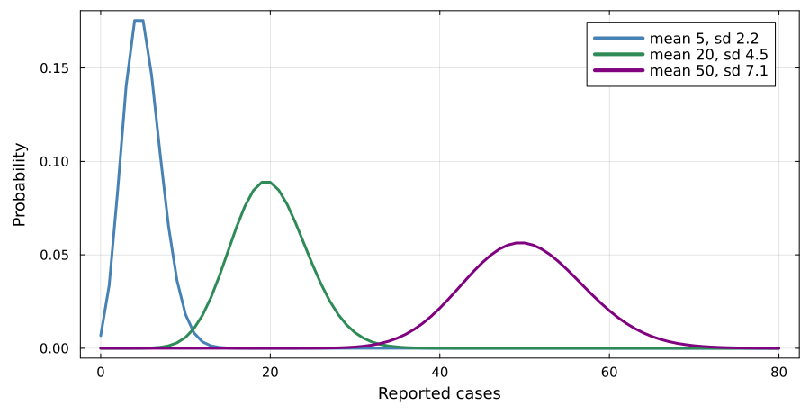
• Observations follow a Poisson distribution around true incidence. The variance equals the mean. With 100 cases, expect a spread of about $\pm 10$.
• Observations at different times are conditionally independent given the trajectory.
• Every case is reported independently with the same probability.

Weekend effects, reporting delays, outbreak investigations and clustered transmission all break these assumptions.

One parameter, so one spread

Overdispersion

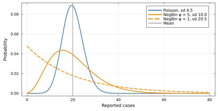
When the data are more variable than Poisson allows, the fix is an observation model with a free variance:

$$y_t \sim \text{NegativeBinomial}(\lambda_t, \phi)$$

• $\phi \to \infty$ recovers the Poisson
• small $\phi$ allows a much wider spread at the same mean

What each model predicts after fitting

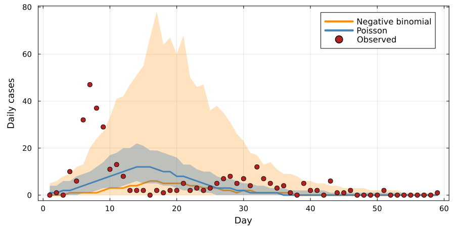
Both fits use the same SIR model on Tristan da Cunha. Only the observation model differs.

Why it matters for inference

An observation model that is too tight makes the posterior too confident.

Day 7 reports 47 cases where the Poisson fit predicts about five. That is near-impossible under Poisson, so the posterior narrows around a trajectory that never reaches it.

Under a negative binomial the same day is merely unusual, so the intervals widen.

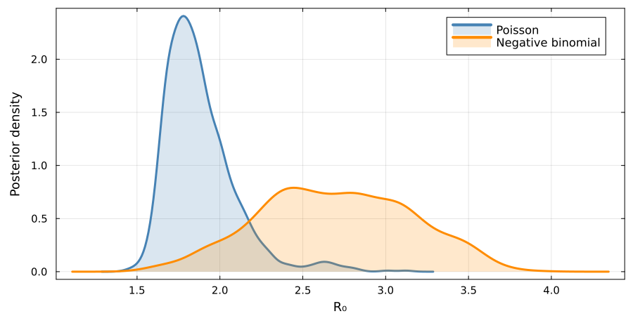
The posteriors disagree about $R_0$

The interval widens and the estimate moves. $D_\mathrm{inf}$ moves too, from about 3.3 days to 6.8.

Likelihood as a distance

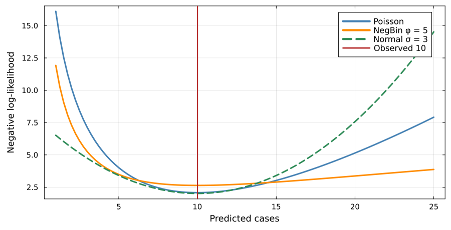
The negative log-likelihood of one observation, as a function of how far it is from the prediction, is a distance function.

• Poisson penalises large relative deviations sharply
• Negative binomial is more forgiving in the tails
• Gaussian penalises absolute deviations symmetrically

Three likelihoods, three distances

The flatter the tail, the less a badly missed day costs. Day 7 costs the Poisson about 66 log units and the negative binomial about 8.

Today’s question

Once you see the likelihood as a distance, an obvious one follows: what if we chose the distance directly?

That is tomorrow morning.

Your Turn

In the practical you will

• fit the Tristan da Cunha data with a Poisson observation model
• check whether its variance assumption actually holds for the data
• refit with a negative binomial and compare
• see the likelihood plotted explicitly as a distance function

Return to the session