Particle MCMC

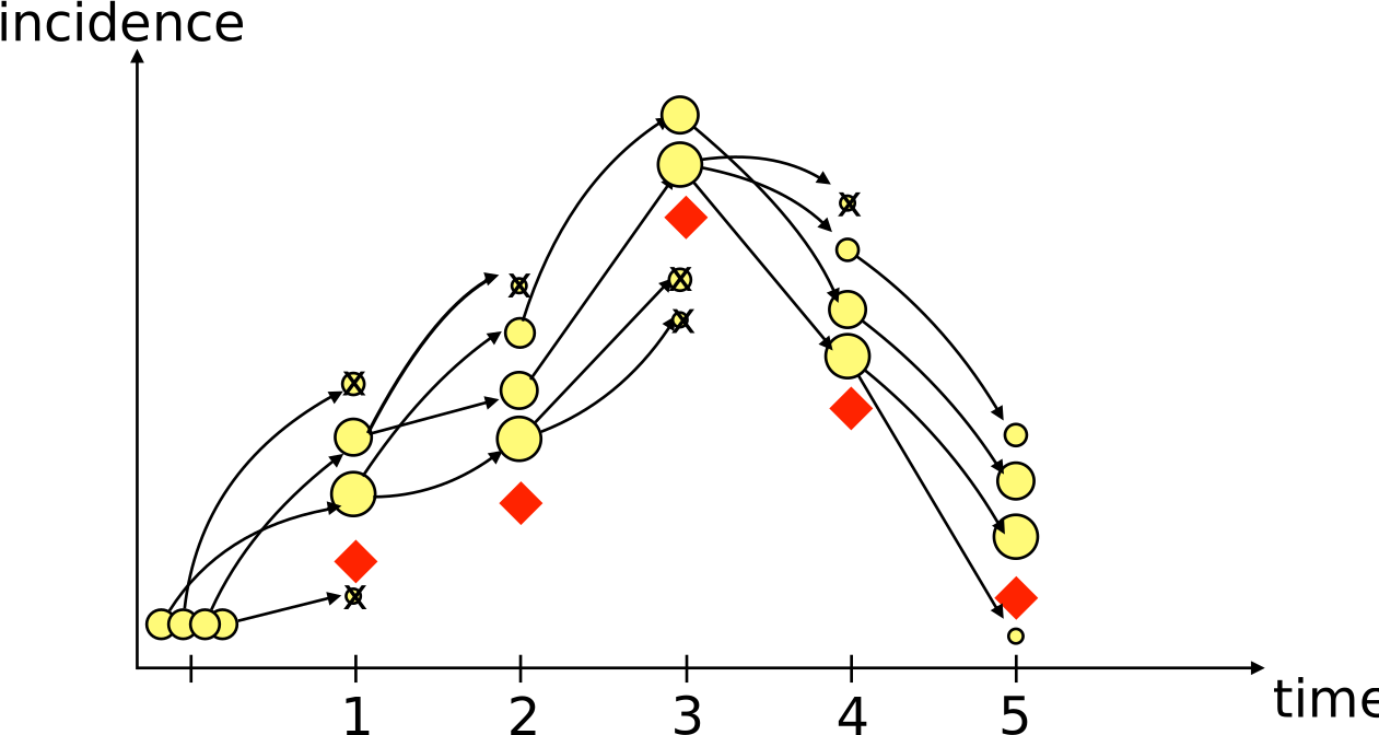
Fitting parameters of stochastic models

Where we got to

$$\hat{p}(y \mid \theta) = \prod_{t} \frac{1}{J}\sum_{j=1}^{J} w_{t,j}$$

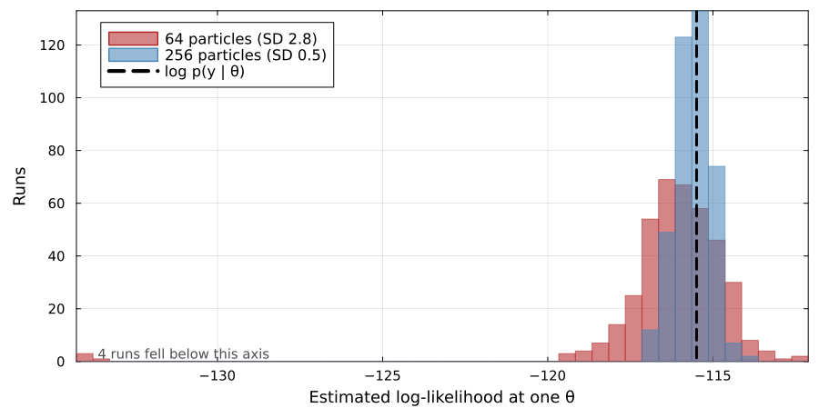
An estimate of the marginal likelihood at one $\theta$. We want the posterior over $\theta$.

Substituting the estimate

We already have an algorithm that explores a posterior using nothing but likelihood evaluations: Metropolis-Hastings.

So: propose $\theta^*$, run a particle filter to get $\hat{p}(y \mid \theta^*)$, and accept or reject as usual.

$$r = \min\left(1, \frac{\hat{p}(y \mid \theta^*)\, p(\theta^*)}{\hat{p}(y \mid \theta)\, p(\theta)}\right)$$

This is particle marginal Metropolis-Hastings (PMMH).

Why should that work at all?

Same $\theta$, same data, 400 runs of the filter — fed into an algorithm derived assuming the exact likelihood.

The reason it works

The estimate is unbiased:

$$\mathbb{E}\big[\hat{p}(y \mid \theta)\big] = p(y \mid \theta)$$

The chain still targets the correct posterior — exactly, not approximately. The noise costs us efficiency, never correctness.

Andrieu et al. (2010) — derived in the appendix

The practical problem

Noise makes the chain sticky

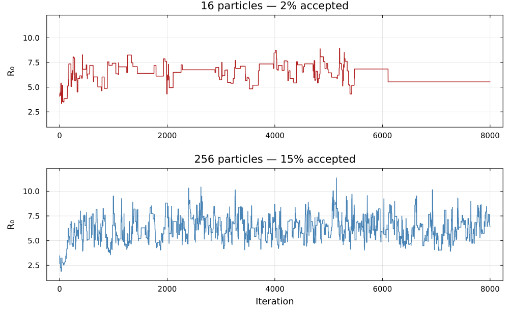
A lucky high estimate sits in the denominator of every later acceptance ratio, so the chain rejects good proposals until something beats it.

Choosing the number of particles

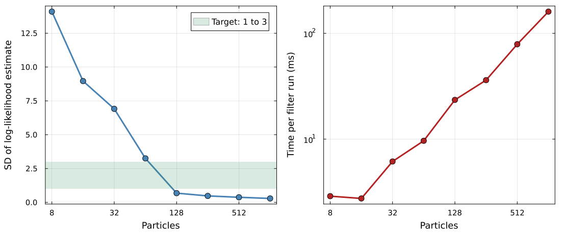
Tune $J$ so the standard deviation of the log likelihood estimate is roughly 1 to 3 at a representative $\theta$.

Measured here at the posterior mean. The estimator is noisier out in the tails of the posterior, which is why the practical uses 256 rather than the 128 this curve appears to license.

Pitt et al. (2012); Doucet et al. (2015)

Why RAM rather than NUTS

• Resampling and discrete events make the likelihood non-differentiable: no gradient to follow.
• The filter returns a different number every run, so there is no fixed surface for HMC to integrate along.

Metropolis-Hastings survives the second because the estimate is unbiased. HMC does not.

So we use robust adaptive Metropolis, which learns the proposal covariance for us (Vihola 2012).

The pay-off

Everything from the deterministic part of the course now carries over to stochastic models:

• posterior distributions over parameters
• credible intervals
• posterior predictive checks

And we get the latent trajectories for free: each accepted $\theta$ comes with a sampled state path, which is state estimation alongside parameter estimation.

Comparing models

Is temporary immunity better described by one compartment or four? No amount of sampling SEITL answers that: you have to fit both.

• Posterior predictive checks: which reproduces the features you care about?
• DIC: the fit at the posterior mean, penalised by how much worse the fit is on average across the posterior

Both ask only for the likelihood of the whole series, which is what the filter returns. DIC is the criterion we can compute here, and a rough one: it approximates predictive accuracy less well than the criteria usually recommended, which need a likelihood term for each observation on its own.

The criterion that is appropriate for model comparison is determined by the structure of the model.

DIC

Deviance, so that smaller is a better fit: $D(\theta) = -2 \log p(y \mid \theta)$.

$$\mathrm{DIC} = D(\bar{\theta}) + 2 p_D, \qquad p_D = \overline{D} - D(\bar{\theta})$$

• $D(\bar{\theta})$: the fit at the posterior mean $\bar{\theta}$
• $\overline{D}$: the fit averaged over the posterior
• $p_D$: how much worse the average is than the fit at the mean, the effective number of parameters

Lower is better, and only the difference between two models means anything.

Your Turn

In the practical you will

• assemble the particle filter and Metropolis-Hastings into PMMH
• run a short chain and see the poor mixing for yourself
• vary the particle count and watch the trade-off appear
• work with a pre-computed long chain, and compare against the deterministic fit
• compare SEITL against SEIT4L, from the pre-computed chains, with DIC and a posterior predictive check

Appendix: why PMMH is exact

Making the randomness explicit

The filter is random only because it consumes random numbers. Collect all of them into one vector $u$:

• the draws that initialise the particles
• the noise that propagates each particle at each step
• the uniforms that drive resampling

Write $m(u)$ for their density. Because the propagation is a deterministic map applied to standard draws, $m$ does not depend on $\theta$.

Given $u$, the filter is a deterministic function:

$$\hat{p}(y \mid \theta) = \hat{p}(y \mid \theta, u)$$

A distribution on the enlarged space

Define a joint density over the pair $(\theta, u)$:

$$\tilde{\pi}(\theta, u) = \frac{p(\theta)\, \hat{p}(y \mid \theta, u)\, m(u)}{p(y)}$$

Integrating $u$ out at fixed $\theta$ averages the estimator over its own randomness, which is exactly what unbiasedness controls:

$$\int \hat{p}(y \mid \theta, u)\, m(u)\, \mathrm{d}u = \mathbb{E}\big[\hat{p}(y \mid \theta)\big] = p(y \mid \theta)$$

This is the only place unbiasedness is used.

The marginal is the posterior

It follows that $\tilde{\pi}$ integrates to one, and that

$$\int \tilde{\pi}(\theta, u)\, \mathrm{d}u = \frac{p(\theta)\, p(y \mid \theta)}{p(y)} = p(\theta \mid y)$$

The $\theta$-marginal of the enlarged target is the posterior we wanted.

PMMH is Metropolis-Hastings on that target

Propose $\theta^*$ from $q(\cdot \mid \theta)$, then fresh random numbers $u^* \sim m(\cdot)$. The Metropolis-Hastings ratio for $\tilde{\pi}$ under that proposal is

$$\underbrace{\frac{p(\theta^*)}{p(\theta)} \cdot \frac{\hat{p}(y \mid \theta^*, u^*)}{\hat{p}(y \mid \theta, u)} \cdot \frac{m(u^*)}{m(u)}}_{\text{target}} \;\cdot\; \underbrace{\frac{q(\theta \mid \theta^*)}{q(\theta^* \mid \theta)} \cdot \frac{m(u)}{m(u^*)}}_{\text{proposal}}$$

The two $m$ factors are reciprocals, so they cancel, leaving

$$\frac{p(\theta^*)\, \hat{p}(y \mid \theta^*, u^*)\, q(\theta \mid \theta^*)}{p(\theta)\, \hat{p}(y \mid \theta, u)\, q(\theta^* \mid \theta)}$$

This is the acceptance ratio we started from. The random numbers never appear in the implementation because their proposal density cancels against their target density.

What the argument gives

• It holds for any number of particles, $J = 1$ included. Correctness never required $J$ to be large.
• The variance of $\hat{p}$ never entered, which is why noise costs efficiency alone.
• $u$ is part of the chain’s state and changes only when a move is accepted. A lucky $u$ is carried until something beats it: the plateaus we saw earlier, seen from the enlarged space.

The condition worth naming is that $\tilde{\pi}$ must be a proper density, so the estimator has to be non-negative and strictly positive wherever the posterior is. Particle filter estimates satisfy this.

Andrieu and Roberts (2009); Andrieu et al. (2010)

Return to the session