Structure and stochasticity

Stochastic models and the state-space view

Where we left off

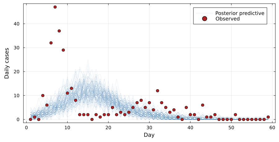
The checks failed

An SIR model fitted to Tristan da Cunha. Too small, too late, too few.

So we change something

The parameters are not the problem. Two changes to the SIR model:

1. Add a mechanism. SIR cannot infect anyone twice, and 92 islanders were. No $R_0$ repairs a structure that forbids it.

2. Add stochasticity. The ODE treats 284 people as a smooth quantity. At that size, chance decides how big the second wave is — or whether there is one.

They are independent. This session makes each in turn.

The state-space view

What we really want to know

We want to find out two things:

1. the parameters of the process, $\theta$
2. the state process, $x$, as opposed to what we observe

We want to do this on the basis of observations (data), $y$.

Why the state needs its own layer

In a deterministic model the state is a function of the parameters: one $\theta$, one trajectory, and $x$ is not something that needs to be separately inferred.

In a stochastic model the same $\theta$ gives a different trajectory every time, so the state has a distribution, $p(x \mid \theta)$.

That extra layer, between the parameters and the data, is what the rest of this session is about.

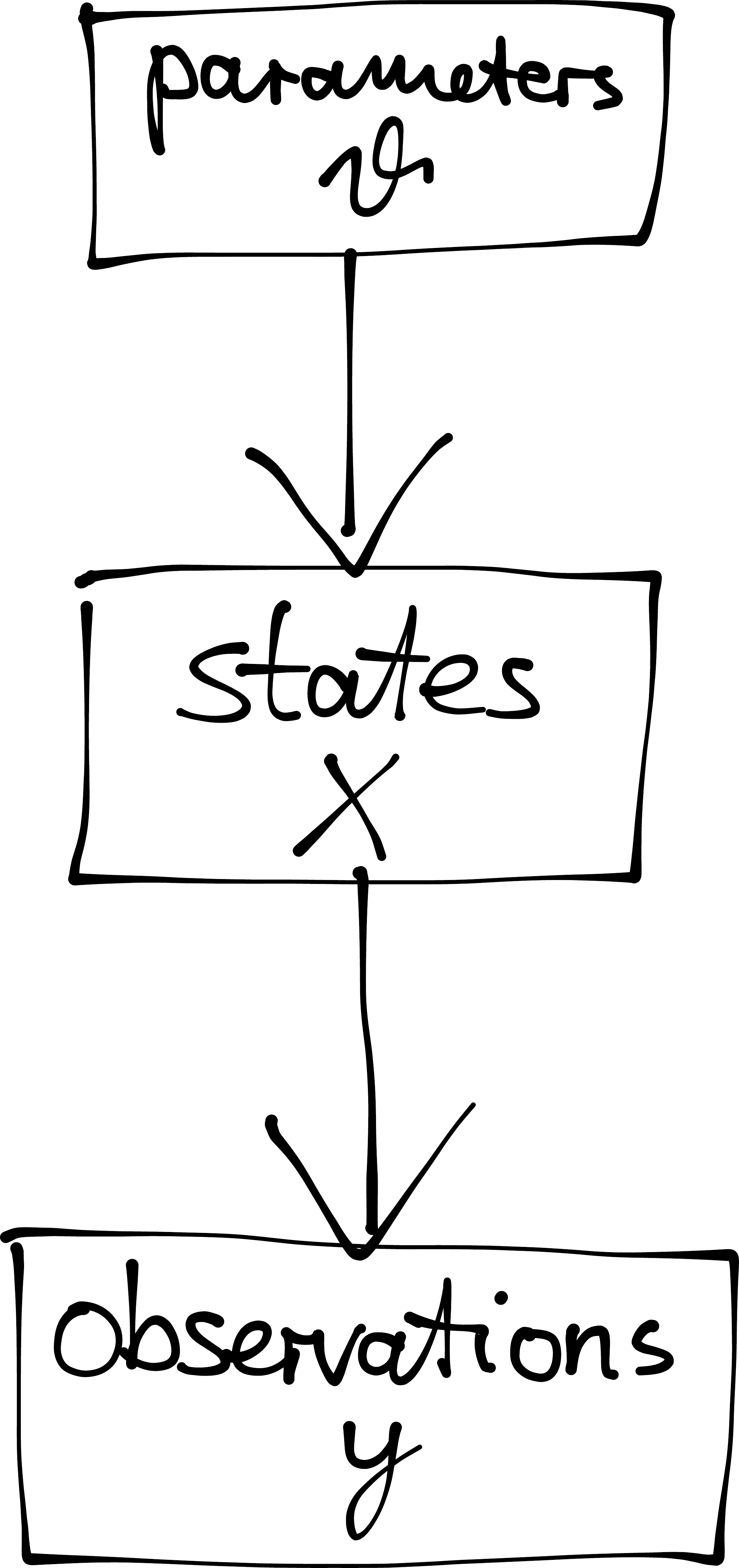
Three layers

Parameters, then states, then observations: each layer depends on the one above. When the states form a time series, a model with this structure is called a state-space model.

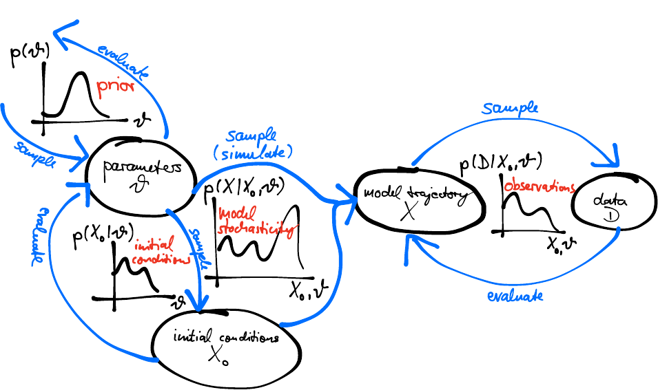
Combining the probabilities

1. prior probabilities of the parameters $$p(\theta)$$
2. model trajectories $$p(x \mid \theta)$$
3. observations $$p(y \mid x, \theta)$$

The joint probability

Applying the chain rule to those three pieces gives

$$p(y, x, \theta) = p(y \mid x, \theta)\, p(x \mid \theta)\, p(\theta)$$

Fitting a state-space model

Doing inference

Set $y$ to the data we observe, and the joint probability gives the posterior

$$p(x, \theta \mid y) = \frac{p(y, x, \theta)}{p(y)}$$

which factorises as

$$p(x, \theta \mid y) = p(\theta \mid y)\, p(x \mid \theta, y)$$

The first factor gives us parameter fitting, the second state estimation.

Parameter estimation

$$p(x, \theta \mid y) = p(\theta \mid y)\, p(x \mid \theta, y)$$

• In a deterministic model, every $\theta$ leads to one possible $x_{\theta}$. In that case

  $$p(x_{\theta}, \theta \mid y) = p(\theta \mid y)$$

• In general we cannot write down a formula for $p(x_{\theta}, \theta, y)$. But we can sample from it.

The model we will fit

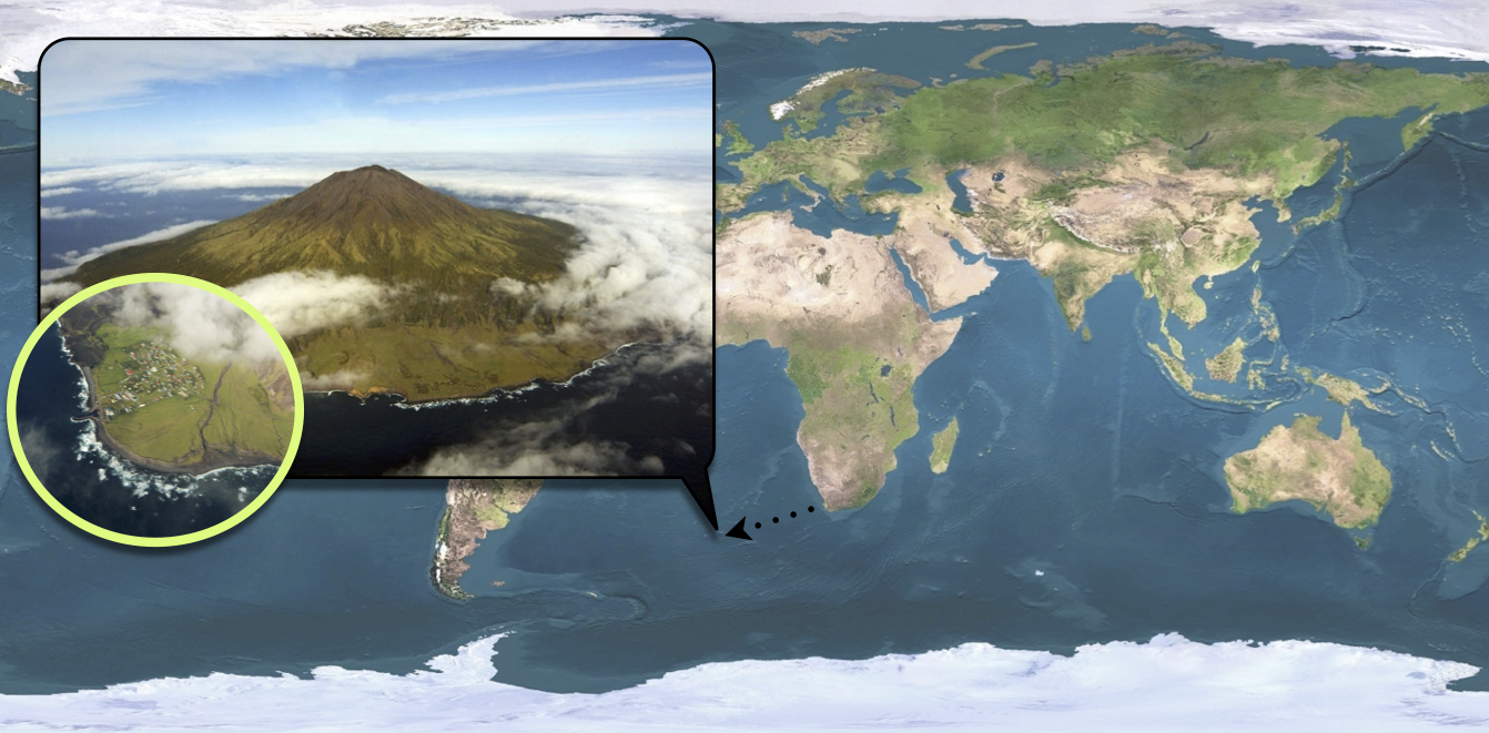
The island

284 people, one ship every few months.

SEITL

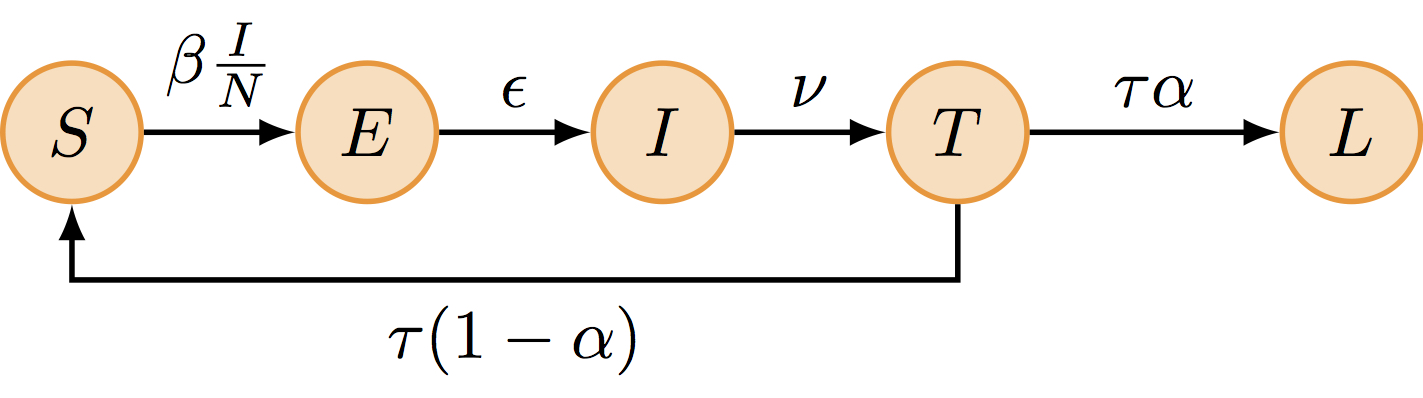
T is temporary immunity, and only a fraction $\alpha$ goes on to L, long-term immunity. The rest return to susceptible and can drive a second wave.

Two independent choices

Model structure — how many compartments, and what flows between them.

Deterministic or stochastic — whether transitions are continuous flows or discrete random events.

These are separate decisions. You can simulate SEITL either way, and the practical does both so you can see the difference.

Why stochastic, here

With 284 people, random events play a relatively large role.

• Individual runs peak days apart
• Some fade out entirely; the deterministic model never does
• The deterministic trajectory is not the average of the stochastic ones

Demographic noise scales roughly as $1/\sqrt{N}$.

Simulating it: Gillespie

The deterministic version solves an ODE. The stochastic version simulates events one at a time.

1. Given the current state, compute the rate of every possible transition
2. Draw the time to the next event from an exponential distribution
3. Pick which event happens, with probability proportional to its rate
4. Update the state, and repeat

Exact, but slow. Every infection and recovery is an individual event.

SEIT4L: why four compartments

A single T compartment means the waiting time in it is exponential, so the most likely thing is to leave immediately.

That is a strange claim about immunity.

Chaining four compartments, each at four times the rate, gives an Erlang waiting time: same mean, but a peak away from zero. Most people stay immune for roughly the average duration.

Your Turn

In the practical you will

• build the SEITL model, which adds the mechanism the checks asked for
• simulate it both deterministically and stochastically
• compare deterministic and stochastic runs of the same model
• see why the stochastic version needs different inference machinery

Return to the session