Model checking and validation

Estimated time: 55 minutes

Slides

Introduction

Where we are: You’ve learned to calculate posteriors (Introduction), sample them with MCMC, and check convergence (Diagnostics). Now we ask: even if the sampler worked, does the model make sense?

You’ve learned how to fit models and diagnose MCMC convergence. But a converged chain doesn’t mean your model is correct - it just means the sampler has explored the posterior properly. This session focuses on a different question: does your model actually describe the data well? We ask it of a real outbreak, on Tristan da Cunha in 1971, which the rest of the course goes on to fit.

Model checking is about building trust in your inferences. A model that doesn’t generate data resembling your observations shouldn’t be trusted to make predictions or inform policy.

Objectives

In this session you will:

1. Use prior predictive checks to validate model specification
2. Use posterior predictive checks to assess model fit
3. Read a posterior predictive p-value near 0 or 1 as the model missing that feature, rather than as a significant test result
4. Interpret residual patterns to diagnose model problems
5. Use simulation-based calibration to check that the inference procedure recovers parameters it was given, and read its rank histogram

Setup

Source file

The source file of this session is located at sessions/model_checking.qmd.

Load libraries

using Random
using Distributions
using DifferentialEquations
using DataFrames
using Plots
using StatsPlots
using Turing
using FlexiChains: @varname ## refer to a model variable by name
using CSV
using DrWatson
using StatsBase

Initialisation

Random.seed!(1234)

TaskLocalRNG()

Load data

The session fits the daily case counts from the Tristan da Cunha outbreak described below.

# Alternatively, you can load directly from GitHub:
# flu_tdc_url = "https://raw.githubusercontent.com/mfiidd/mfiidd/main/data/flu_tdc_1971.csv"
# flu_tdc = CSV.read(download(flu_tdc_url), DataFrame)
flu_tdc = CSV.read(datadir("flu_tdc_1971.csv"), DataFrame)

59×3 DataFrame

34 rows omitted

Row	date	time	obs
	Date	Int64	Int64
1	1971-08-13	1	0
2	1971-08-14	2	1
3	1971-08-15	3	0
4	1971-08-16	4	10
5	1971-08-17	5	6
6	1971-08-18	6	32
7	1971-08-19	7	47
8	1971-08-20	8	37
9	1971-08-21	9	29
10	1971-08-22	10	11
11	1971-08-23	11	13
12	1971-08-24	12	8
13	1971-08-25	13	2
⋮	⋮	⋮	⋮
48	1971-09-29	48	0
49	1971-09-30	49	0
50	1971-10-01	50	0
51	1971-10-02	51	2
52	1971-10-03	52	0
53	1971-10-04	53	0
54	1971-10-05	54	0
55	1971-10-06	55	0
56	1971-10-07	56	0
57	1971-10-08	57	0
58	1971-10-09	58	0
59	1971-10-10	59	1

Tristan da Cunha outbreak

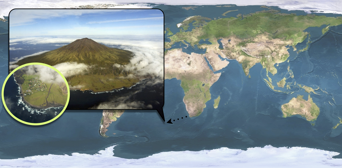
Tristan da Cunha is a volcanic island in the South Atlantic Ocean. It has been inhabited since the $19^{th}$ century and in 1971, the 284 islanders were living in the single village of the island: Edinburgh of the Seven Seas. Whereas the internal contacts were typical of close-knit village communities, contacts with the outside world were infrequent and mostly due to fishing vessels that occasionally took passengers to or from the island. These ships were often the cause of introduction of new diseases into the population. As for influenza, no outbreak had been reported since an epidemic of A/H1N1 in 1954. In this context of a small population with limited immunity against influenza, an unusual epidemic occurred in 1971, 3 years after the global emergence of the new subtype A/H3N2.

On August 13, a ship returning from Cape Town landed five islanders on Tristan da Cunha. Three of them had developed acute respiratory disease during the 8-day voyage and the other two presented similar symptoms immediately after landing. Various family gatherings welcomed their disembarkation and in the ensuing days an epidemic started to spread rapidly throughout the whole island population. After three weeks of propagation, while the epidemic was declining, some islanders developed second episodes of illness and a second peak of cases was recorded. The epidemic faded out after this second wave and lasted a total of 59 days. Despite the lack of virological data, serological evidence indicates that all episodes of illness were due to influenza A/H3N2.

Among the 284 islanders, 273 (96%) experienced at least one episode of illness and 92 (32%) experienced two, which is remarkable for influenza. Unfortunately, only 312 of the 365 attacks (85%) are known to within a single day of accuracy and constitute the dataset reported by Mantle & Tyrrell in 1973.

The daily incidence data, loaded in the setup above, look like this:

# Display first few rows
first(flu_tdc, 6)

6×3 DataFrame

Row	date	time	obs
	Date	Int64	Int64
1	1971-08-13	1	0
2	1971-08-14	2	1
3	1971-08-15	3	0
4	1971-08-16	4	10
5	1971-08-17	5	6
6	1971-08-18	6	32

# Plot daily observed incidence
scatter(
    flu_tdc.time, flu_tdc.obs,
    xlabel = "Time (days)", ylabel = "Daily incidence",
    label = "Observed cases", markersize = 4, color = :red,
    title = "Tristan da Cunha 1971 Influenza Outbreak"
)

The two waves are the reason this dataset is worth fitting in a session about model checking. A simple SIR model has no way to infect anybody twice, and 312 attacks in a population of 284 means somebody was. We fit it anyway, and spend the session on what the checks say about a model we already have reason to doubt.

The Bayesian workflow

Model checking isn’t a one-time step at the end - it’s part of the process. Gelman et al. (2020) describe this as the “Bayesian workflow”:

1. Specify model - choose structure, priors, likelihood
2. Prior predictive check - do simulations from priors look reasonable?
3. Fit model - run MCMC or other inference
4. Diagnose sampler - check convergence (previous session)
5. Posterior predictive check - does the fitted model generate realistic data?
6. Iterate - if checks fail, revise the model

So far we’ve focused on steps 1, 3, and 4. This session covers the checking steps (2 and 5) that tell you whether the model itself makes sense - not just whether the sampler worked.

Prior predictive checks

Before fitting any data, you should ask: do my priors make sense? Prior predictive checking simulates data purely from your prior assumptions, without conditioning on observations.

Let’s use the SIR model from the introduction:

function sir_ode!(du, u, p, t)
    R_0, D_inf = p
    β = R_0 / D_inf
    ν = 1.0 / D_inf
    S, I, R, C = u
    N = S + I + R

    du[1] = -β * S * I / N
    du[2] = β * S * I / N - ν * I
    du[3] = ν * I
    du[4] = β * S * I / N  # Cumulative incidence
end

sir_prob = ODEProblem(sir_ode!, zeros(4), (0.0, 1.0), [2.5, 5.0])

function simulate_sir(R_0, D_inf, init_state, times)
    times_vec = collect(times)
    u0 = [init_state[:S], init_state[:I], init_state[:R], 0.0]
    prob = remake(
        sir_prob, u0 = u0, p = [R_0, D_inf],
        tspan = (times_vec[1], times_vec[end])
    )
    sol = solve(prob, Tsit5(), saveat=times_vec)

    # The model tracks cumulative incidence, so daily incidence is the difference
    # between consecutive days.
    inc_cumulative = sol[4, :]
    inc_daily = diff(inc_cumulative)

    return (time=times_vec, S=sol[1, :], I=sol[2, :], R=sol[3, :], inc=inc_daily)
end

simulate_sir (generic function with 1 method)

The compartments are returned alongside incidence. Incidence is the difference between consecutive days, so it has one value fewer than the compartments do.

Now let’s define a model with priors and sample from the prior predictive distribution:

@model function sir_model(times, init_state, n_obs)
    # Priors
    R_0 ~ Uniform(0.5, 10.0)
    D_inf ~ Uniform(1.0, 14.0)
    ρ ~ Uniform(0.0, 1.0)  # Reporting rate

    # Simulate.
    traj = simulate_sir(R_0, D_inf, init_state, times)

    # Likelihood
    lambdas = [max(ρ * traj.inc[i], 1e-10) for i in 1:n_obs]
    obs ~ arraydist(Poisson.(lambdas))

    return traj
end

sir_model (generic function with 2 methods)

The return statement plays no part in the fit. It hands back the whole trajectory, so every compartment the model simulated is available afterwards through returned(), for prior draws and posterior draws alike.

TipWhy max(..., 1e-10) everywhere?

You’ll see max(value, 1e-10) throughout the course wherever we create a Poisson distribution. Poisson(λ) requires λ > 0 — passing exactly zero causes an error. In practice, the model can produce zero expected incidence (e.g. before the epidemic starts or after it ends), and numerical noise from the ODE solver can even produce tiny negative values. The max(..., 1e-10) guard ensures we always pass a valid (tiny but positive) rate. The value 1e-10 is small enough to be effectively zero for all practical purposes.

# Prior predictive sampling.
times = 0.0:1.0:59.0

## The island as the ship lands, at the start of day 1. Of the five islanders it
## brought back, three had been ill during the eight day voyage and are past their
## infectious period, so they start recovered; the two who fell ill on landing
## start infectious. N = 284, the island population
init_state = Dict(:S => 279.0, :I => 2.0, :R => 3.0)
N = init_state[:S] + init_state[:I] + init_state[:R]

# Sample from priors (no data conditioning — obs will be sampled from the model)
prior_model = sir_model(times, init_state, length(times) - 1)
prior_samples = sample(prior_model, Prior(), 200, progress=false)
prior_trajs = vec(returned(prior_model, prior_samples))

200-element Vector{@NamedTuple{time::Vector{Float64}, S::Vector{Float64}, I::Vector{Float64}, R::Vector{Float64}, inc::Vector{Float64}}}:
 (time = [0.0, 1.0, 2.0, 3.0, 4.0, 5.0, 6.0, 7.0, 8.0, 9.0  …  50.0, 51.0, 52.0, 53.0, 54.0, 55.0, 56.0, 57.0, 58.0, 59.0], S = [279.0, 271.2196079978836, 243.45285531068504, 174.31128019927533, 89.42899478028426, 39.70394758609245, 19.33865657701575, 11.131002936776182, 7.45789011792848, 5.620921963197272  …  2.976193160055852, 2.976193044890639, 2.976192965279472, 2.976192912555366, 2.9761928772977093, 2.9761928512550084, 2.9761928329682683, 2.9761928212416033, 2.9761928141181455, 2.976192808947291], I = [2.0, 8.048330796109294, 29.200774661536137, 77.88292540517412, 121.89370907754933, 121.90904143460781, 98.24593265412008, 72.63441277612347, 51.78757147130413, 36.29977416208964  …  7.129186428687378e-6, 4.874618846496592e-6, 3.3160860138761322e-6, 2.2839161051821406e-6, 1.593683600934939e-6, 1.0838505232183595e-6, 7.258544345782779e-7, 4.96283713881168e-7, 3.568291136701493e-7, 2.556002781677181e-7], R = [3.0, 4.732061206007152, 11.346370027778912, 31.805794395550635, 72.67729614216653, 122.38701097929986, 166.4154107688643, 200.23458428710046, 224.7545384107675, 242.07930387471322  …  281.02379971075777, 281.02380208049055, 281.02380371863455, 281.02380480352855, 281.0238055290187, 281.0238060648945, 281.0238064411773, 281.0238066824747, 281.0238068290528, 281.02380693545246], inc = [7.780392002116446, 27.7667526871986, 69.14157511140972, 84.88228541899106, 49.7250471941918, 20.365291009076685, 8.207653640239585, 3.6731128188476987, 1.8369681547312098, 1.0068402360302002  …  1.63767481353716e-7, 1.1516522135934792e-7, 7.961114079080289e-8, 5.272414682622184e-8, 3.525764213918592e-8, 2.604269866424147e-8, 1.828675522119738e-8, 1.1726626780728111e-8, 7.123446721379878e-9, 5.170875283511123e-9])
 (time = [0.0, 1.0, 2.0, 3.0, 4.0, 5.0, 6.0, 7.0, 8.0, 9.0  …  50.0, 51.0, 52.0, 53.0, 54.0, 55.0, 56.0, 57.0, 58.0, 59.0], S = [279.0, 277.5732736918292, 275.3394005831503, 271.87112946177587, 266.5561838181847, 258.5718272646605, 246.9278254145322, 230.6561496768192, 209.21946820458643, 183.0456650419836  …  1.491293477115021, 1.4762696236109838, 1.4628518141928188, 1.4508528053730982, 1.4401093798656874, 1.4304823916085683, 1.4218531958594072, 1.4141148821584735, 1.407171302863661, 1.400937146461286], I = [2.0, 3.1579624734832255, 4.968235793146452, 7.771975381426286, 12.051933232117237, 18.442029872490018, 27.670502364749936, 40.368708809966044, 56.692189900092814, 75.85929164426655  …  5.271360008175672, 4.755422840992256, 4.290021961235766, 3.8701645037053947, 3.491289077943448, 3.149307360865508, 2.8407460163814653, 2.5623910381705093, 2.311289199305826, 2.0847610765352376], R = [3.0, 3.268763834687561, 3.692363623703281, 4.356895156797842, 5.391882949698022, 6.986142862849473, 9.401672220717822, 12.975141513214716, 18.088341895320724, 25.095043313749837  …  277.2373465147092, 277.7683075353967, 278.24712622457133, 278.67898269092143, 279.0686015421908, 279.4202102475258, 279.73740078775904, 280.0234940796709, 280.2815394978304, 280.51430177700337], inc = [1.4267263081707862, 2.233873108678948, 3.468271121374395, 5.31494564359113, 7.984356553524231, 11.644001850128273, 16.271675737713004, 21.436681472232785, 26.173803162602823, 29.200631743838528  …  0.016841167278641933, 0.015023853504033013, 0.013417809418172055, 0.011999008819714163, 0.010743425507428128, 0.009626988257139146, 0.00862919574916532, 0.00773831370094058, 0.006943579294784286, 0.006234156402399549])
 (time = [0.0, 1.0, 2.0, 3.0, 4.0, 5.0, 6.0, 7.0, 8.0, 9.0  …  50.0, 51.0, 52.0, 53.0, 54.0, 55.0, 56.0, 57.0, 58.0, 59.0], S = [279.0, 277.7967927619014, 276.5937719251444, 275.3940637451593, 274.2007489111558, 273.01683064266655, 271.8451958004298, 270.68860483920776, 269.5496599960447, 268.4307827402944  …  245.96627363734598, 245.8272733413285, 245.697081519665, 245.57517675415315, 245.46105855099748, 245.35424734080942, 245.2542844786074, 245.16073224381668, 245.07317384026962, 244.99122693426764], I = [2.0, 2.0109770399414004, 2.016778512394979, 2.017366963637672, 2.012758963195239, 2.003024463769101, 1.9882837959318573, 1.9687059075152074, 1.9445056400085992, 1.9159381671708884  …  0.27080965913029126, 0.2538717203903144, 0.23792565593973677, 0.2229235028385712, 0.2088179161580119, 0.19556216898043507, 0.1831101523993977, 0.17141637551963862, 0.16043596545707797, 0.1501268533623714], R = [3.0, 4.192230198157223, 5.389449562460676, 6.588569291203031, 7.786492125648969, 8.980144893564367, 10.166520403638389, 11.342689253277085, 12.505834363946773, 13.653279092534747  …  37.76291670352381, 37.91885493828127, 38.064992824395325, 38.20189974300834, 38.330123532844596, 38.450190490210225, 38.5626053689933, 38.66785138066374, 38.766390194273384, 38.85864621237004], inc = [1.2032072380986236, 1.2030208367570314, 1.1997081799850484, 1.1933148340035058, 1.1839182684892595, 1.1716348422367782, 1.1565909612220455, 1.1389448431630829, 1.1188772557502613, 1.0965910234711682  …  0.14835111298081216, 0.13900029601749253, 0.1301918216634732, 0.12190476551185014, 0.11411820315569088, 0.10681121018806294, 0.09996286220203388, 0.09355223479067831, 0.0875584035470851, 0.08194690600195287])
 (time = [0.0, 1.0, 2.0, 3.0, 4.0, 5.0, 6.0, 7.0, 8.0, 9.0  …  50.0, 51.0, 52.0, 53.0, 54.0, 55.0, 56.0, 57.0, 58.0, 59.0], S = [279.0, 277.6306083394718, 275.52541856162173, 272.3137362240301, 267.47067671768855, 260.2940984920965, 249.92879255974165, 235.49901806489098, 216.39949963356497, 192.7257615274843  …  1.9078617226044112, 1.889059801264694, 1.8722651826935626, 1.857259013409704, 1.8438450136799132, 1.831845309019446, 1.8211004301920197, 1.811469313209812, 1.8028296334094946, 1.795078664833873], I = [2.0, 3.0991619048260866, 4.7863123272940165, 7.354039691279066, 11.211541288833219, 16.89436089087117, 25.027903642332298, 36.19163134661303, 50.64604798070675, 67.95639412222354  …  5.319617578985831, 4.794524440886815, 4.320893961879142, 3.8939135980711317, 3.509137577933518, 3.162443945344954, 2.85003455959201, 2.5684350953691646, 2.3145120349630997, 2.085628409102962], R = [3.0, 3.270229755702121, 3.6882691110842676, 4.332224084690834, 5.317781993478264, 6.811540617032306, 9.043303797926047, 12.309350588496004, 16.954452385728302, 23.317844350292173  …  276.7725206984098, 277.3164157578485, 277.8068408554273, 278.2488273885192, 278.6470174083866, 279.0057107456356, 279.328865010216, 279.62009559142103, 279.88265833162745, 280.11929292606317], inc = [1.369391660528208, 2.1051897778500757, 3.2116823375916166, 4.843059506341582, 7.176578225591998, 10.365305932354861, 14.429774494850697, 19.099518431325997, 23.67373810608067, 27.101943462332954  …  0.02106976277582362, 0.018801921339729688, 0.01679461857111164, 0.01500616928387899, 0.01341399972977797, 0.011999704660468069, 0.010744878827438242, 0.009631116982177446, 0.008639679800296562, 0.007750968575635397])
 (time = [0.0, 1.0, 2.0, 3.0, 4.0, 5.0, 6.0, 7.0, 8.0, 9.0  …  50.0, 51.0, 52.0, 53.0, 54.0, 55.0, 56.0, 57.0, 58.0, 59.0], S = [279.0, 276.6076098023339, 271.9794302510749, 263.26308495650085, 247.64511171953353, 221.99294199850596, 185.28253106031673, 141.744125232699, 99.95817890354103, 66.79879198544108  …  1.3914967664130664, 1.38989220427275, 1.388517744837629, 1.3873393461309054, 1.3863302667191448, 1.3854668690923042, 1.3847279997745963, 1.3840949893244907, 1.3835521212225992, 1.3830870219153848], I = [2.0, 3.9387733523218444, 7.6781673294971124, 14.678797230896587, 27.07541039267602, 46.9677245358855, 74.15647870246859, 103.58572620725928, 126.97473378836968, 138.90571625983617  …  0.4142534917483734, 0.35508238262621394, 0.30434273402931616, 0.26079965397663296, 0.22348235231298477, 0.19152993444117114, 0.1641699647408136, 0.14071846656835652, 0.12059774050039224, 0.10335295346179638], R = [3.0, 3.4536168453442397, 4.342402419427998, 6.05811781260256, 9.279477887790451, 15.039333465608545, 24.560990237214682, 38.67014856004172, 57.0670873080893, 78.29549175472276  …  282.1942497418386, 282.25502541310107, 282.3071395211331, 282.3518609998925, 282.3901873809679, 282.42300319646654, 282.4511020354846, 282.4751865441072, 282.49585013827704, 282.51356002462285], inc = [2.3923901976660837, 4.628179551259025, 8.716345294574037, 15.617973236967318, 25.65216972102758, 36.71041093818924, 43.53840582761772, 41.78594632915795, 33.159386918099955, 22.972383588154514  …  0.0018756945261770852, 0.001604562140357757, 0.0013744594350555417, 0.0011783987067701673, 0.0010090794117445512, 0.0008633976268583865, 0.0007388693176721972, 0.0006330104500875677, 0.0005428681018884163, 0.00046509930723459547])
 (time = [0.0, 1.0, 2.0, 3.0, 4.0, 5.0, 6.0, 7.0, 8.0, 9.0  …  50.0, 51.0, 52.0, 53.0, 54.0, 55.0, 56.0, 57.0, 58.0, 59.0], S = [279.0, 275.4812912074287, 266.7478321694855, 246.54432084130437, 206.52091237070866, 146.86799685567826, 86.72522833117483, 45.05953031282288, 22.45906264196881, 11.400385280631722  …  0.028530042599278965, 0.028364672892666375, 0.02821812807779206, 0.028088277025132915, 0.02797319706230174, 0.02787115123764986, 0.02778058832026715, 0.02770014292442904, 0.027628669714351642, 0.02756517133311465], I = [2.0, 5.132813688598746, 12.886767420755412, 30.69555389225339, 65.3333137469209, 114.62180930915206, 158.74685510693035, 180.5080652993984, 181.94056179366186, 172.38666142045585  …  1.6140965842031139, 1.4375215627761702, 1.2801828253377237, 1.140071306487238, 1.0153445684287303, 0.904313997309262, 0.8054448032189365, 0.7173561853172606, 0.6388752975143573, 0.5689804829904912], R = [3.0, 3.3858951039725294, 4.3654004097590615, 6.76012526644221, 12.145773882370422, 22.51019383516969, 38.527916561894806, 58.43240438777874, 79.60037556436933, 100.21295329891242  …  282.3573733731977, 282.5341137643312, 282.69159904658454, 282.8318404164877, 282.95668223450906, 283.06781485145314, 283.16677460846086, 283.2549436717584, 283.3334960327714, 283.4034543456765], inc = [3.518708792571276, 8.733459037943195, 20.203511328181122, 40.023408470595705, 59.652915515030415, 60.142768524503424, 41.66569801835195, 22.600467670854073, 11.058677361337118, 5.339654586362542  …  0.00018672876308301056, 0.00016536970656488847, 0.00014654481486786608, 0.0001298510526339669, 0.00011507996288173672, 0.00010204582463302359, 9.05629173644229e-5, 8.044539589491251e-5, 7.147321008460494e-5, 6.349838122332585e-5])
 (time = [0.0, 1.0, 2.0, 3.0, 4.0, 5.0, 6.0, 7.0, 8.0, 9.0  …  50.0, 51.0, 52.0, 53.0, 54.0, 55.0, 56.0, 57.0, 58.0, 59.0], S = [279.0, 278.7631703938522, 278.51644441493994, 278.2594443996058, 277.99178142542377, 277.71305525765655, 277.4228543392885, 277.1207557913572, 276.8063256742448, 276.4791185248928  …  245.77817252504022, 244.4731067627119, 243.13881174322285, 241.77559384118274, 240.3838263901493, 238.96394968262823, 237.51647097007316, 236.04196446288572, 234.54107133041555, 233.0144997009602], I = [2.0, 2.0854865608936075, 2.1744085307284826, 2.2668846159950693, 2.363035921807473, 2.462985846453292, 2.566859788953391, 2.674785126986817, 2.7868908897998046, 2.9033079590221167  …  12.627209104204045, 12.983444478068932, 13.342405234083252, 13.70359907997965, 14.066508098160678, 14.430588745698776, 14.795271854336315, 15.159962630485555, 15.524040655228676, 15.886859884317753], R = [3.0, 3.1513430452541864, 3.309147054331549, 3.473670984399112, 3.645182652768764, 3.8239588958901405, 4.010285871758108, 4.204459081655937, 4.406783435955364, 4.617573516085086  …  25.59461837075567, 26.54344875921909, 27.518783022693825, 28.520807078837525, 29.549665511689952, 30.605461571672922, 31.688257175590454, 32.79807290662864, 33.93488801435571, 35.09864041472199], inc = [0.23682960614779436, 0.24672597891223774, 0.25700001533414935, 0.26766297418205653, 0.2787261677671953, 0.2902009183680656, 0.30209854793125546, 0.31443011711241486, 0.32720714935203477, 0.34044103363976586  …  1.2755916971832058, 1.3050657623283115, 1.3342950194890548, 1.3632179020400983, 1.3917674510334521, 1.4198767075210696, 1.4474787125550677, 1.474506507187428, 1.500893132470189, 1.5265716294553613])
 (time = [0.0, 1.0, 2.0, 3.0, 4.0, 5.0, 6.0, 7.0, 8.0, 9.0  …  50.0, 51.0, 52.0, 53.0, 54.0, 55.0, 56.0, 57.0, 58.0, 59.0], S = [279.0, 254.79240141422218, 127.33128004014421, 25.415104350838487, 5.717253435035818, 1.9787297459013333, 0.9656534288428873, 0.5980190689752016, 0.43491361974704096, 0.3520501323808826  …  0.23242836377395062, 0.23242836222135418, 0.23242836131893693, 0.23242836075780854, 0.23242836025822466, 0.23242835989353128, 0.23242835968637518, 0.23242835961024427, 0.23242835959244357, 0.2324283595315195], I = [2.0, 22.613493857835877, 122.60539609989137, 160.71639968303785, 121.34783598078769, 83.06839649346254, 55.667903237593315, 37.06272151342733, 24.61160682135283, 16.323253418341377  …  7.475728048736049e-7, 4.846073895221485e-7, 3.3176372915366213e-7, 2.367246434423501e-7, 1.5210942421802398e-7, 9.03407977824029e-8, 5.525448124992953e-8, 4.2360087367594486e-8, 3.934515835862917e-8, 2.9026365838605944e-8], R = [3.0, 6.594104727941945, 34.063323859964406, 97.86849596612366, 156.9349105841765, 198.95287376063612, 227.36644333356384, 246.33925941759748, 258.95347955890014, 267.3246964492778  …  283.76757088865327, 283.7675711531713, 283.7675713069173, 283.76757140251755, 283.7675714876323, 283.76757154976565, 283.76757158505916, 283.7675715980297, 283.7675716010624, 283.7675716114421], inc = [24.20759858577782, 127.46112137407798, 101.9161756893057, 19.69785091580266, 3.7385236891345244, 1.0130763170583919, 0.36763435986767945, 0.16310544922816916, 0.08286348736618265, 0.046045304231597584  …  2.401804977125721e-9, 1.5526211427641101e-9, 9.023892744153272e-10, 5.611582309938967e-10, 4.995968083676416e-10, 3.647073754109442e-10, 2.071374183287844e-10, 7.611333785462193e-11, 1.779199010343291e-11, 6.093614501878619e-11])
 (time = [0.0, 1.0, 2.0, 3.0, 4.0, 5.0, 6.0, 7.0, 8.0, 9.0  …  50.0, 51.0, 52.0, 53.0, 54.0, 55.0, 56.0, 57.0, 58.0, 59.0], S = [279.0, 268.0757489554422, 217.49332560116648, 106.39105750328154, 31.930087955728194, 9.405139201847172, 3.3502259582362917, 1.4638456984346853, 0.7613446346015362, 0.4557542891437623  …  0.07231640301004964, 0.07231524344473983, 0.07231433538401477, 0.07231362644524929, 0.07231307400758158, 0.07231264220233453, 0.0723123040811703, 0.07231204046014814, 0.07231183504083737, 0.07231167428526084], I = [2.0, 11.565449321889954, 55.03460787098207, 141.8107629864477, 175.3364248610695, 156.28265697636894, 127.22139019066373, 100.94209995445344, 79.40483840865434, 62.24872747836305  …  0.002489215387820143, 0.0019448847459749413, 0.0015186109532454336, 0.0011858077798816912, 0.0009264699850556449, 0.000723760873950584, 0.0005650304927153932, 0.0004412735387246273, 0.00034483908771867005, 0.0002693719203707216], R = [3.0, 4.358801722667839, 11.47206652785143, 35.798179510270714, 76.73348718320227, 118.31220382178385, 153.42838385109997, 181.59405434711186, 203.8338169567441, 221.29551823249318  …  283.9251943816021, 283.9257398718093, 283.9261670536627, 283.92650056577486, 283.92676045600734, 283.9269635969237, 283.9271226654261, 283.9272466860011, 283.92734332587145, 283.9274189537944], inc = [10.924251044557792, 50.58242335427574, 111.10226809788495, 74.46096954755333, 22.524948753881006, 6.0549132436108835, 1.8863802598015695, 0.7025010638332105, 0.30559034545774466, 0.15089403342335572  …  1.4860098644930986e-6, 1.1595652722462546e-6, 9.080607696887455e-7, 7.089387850101048e-7, 5.524376547327847e-7, 4.318052333474043e-7, 3.381211399755557e-7, 2.636210183482035e-7, 2.0541932599371648e-7, 1.6075557596195722e-7])
 (time = [0.0, 1.0, 2.0, 3.0, 4.0, 5.0, 6.0, 7.0, 8.0, 9.0  …  50.0, 51.0, 52.0, 53.0, 54.0, 55.0, 56.0, 57.0, 58.0, 59.0], S = [279.0, 278.01662886364267, 276.89439818314446, 275.616770376064, 274.166185878153, 272.52431290764605, 270.67235511724834, 268.5916396072138, 266.2640981013046, 263.6729585773407  …  131.86089657702462, 131.32141634726761, 130.83868560347534, 130.40729366828384, 130.02207498365772, 129.67810911089023, 129.37072073060313, 129.0954796427468, 128.84820076660023, 128.62618405335684], I = [2.0, 2.293062848338909, 2.6245189595602803, 2.9979616350113596, 3.41686357230807, 3.8843986909991917, 4.403240189911528, 4.975239896827065, 5.601183723396776, 6.280439998314164  …  2.613268550307193, 2.350963695095113, 2.1132976749309313, 1.8985687173040193, 1.7050196363299444, 1.5308378327504668, 1.37415529393354, 1.2330485938733118, 1.1055388931901204, 0.9903886035293494], R = [3.0, 3.690308288018438, 4.481082857295273, 5.385267988924678, 6.41695054953893, 7.591288401354778, 8.924404692840126, 10.433120495959168, 12.134718175298564, 14.046601424345123  …  149.52583487266818, 150.32761995763727, 151.0480167215937, 151.69413761441214, 152.2729053800123, 152.7910530563593, 153.25512397546333, 153.67147176337988, 154.04626034020964, 154.3834273431138], inc = [0.9833711363573467, 1.1222306804982058, 1.2776278070804854, 1.4505844979109606, 1.6418729705069701, 1.8519577903976856, 2.0807155100345778, 2.327541505909105, 2.5911395239639496, 2.8688462292023207  …  0.6018855124142704, 0.5394802297570038, 0.4827307437922741, 0.431391935191499, 0.38521868462612474, 0.3439658727674839, 0.307388380287108, 0.2752410878563296, 0.24727887614656652, 0.22201671324339145])
 ⋮
 (time = [0.0, 1.0, 2.0, 3.0, 4.0, 5.0, 6.0, 7.0, 8.0, 9.0  …  50.0, 51.0, 52.0, 53.0, 54.0, 55.0, 56.0, 57.0, 58.0, 59.0], S = [279.0, 278.4646896958991, 277.83424122481085, 277.0924407858149, 276.2205789041915, 275.19717890077794, 273.9977139541854, 272.5944008757469, 270.95596836786183, 269.0476907694337  …  32.26933228050557, 30.831665606072587, 29.527450433646706, 28.342781552962016, 27.26524902737033, 26.283938193841262, 25.38942754785099, 24.573180325948467, 23.82732488521108, 23.144994845600227], I = [2.0, 2.3609932860451375, 2.7857139629943286, 3.2848516920057613, 3.870672127782096, 4.557160557305914, 5.3601522507277695, 6.297403469838267, 7.388644055171384, 8.655413134653188  …  52.98430188091042, 50.2854594442886, 47.665982786120885, 45.13324087025882, 42.69267696399347, 40.34780863805573, 38.10023072700012, 35.95051634291626, 33.89872413958704, 31.9439137727254], R = [3.0, 3.174317018055749, 3.3800448121948112, 3.622707522179348, 3.9087489680264147, 4.245660541916136, 4.64213379508683, 5.108195654414798, 5.655387576966778, 6.296896095913103  …  198.74636583858398, 202.8828749496388, 206.8065667802324, 210.52397757677915, 214.04207400863618, 217.368253168103, 220.51034172514886, 223.47630333113523, 226.27395097520184, 228.91109138167434], inc = [0.5353103041008874, 0.6304484710882529, 0.7418004389959698, 0.871861881623401, 1.0234000034135398, 1.19946494659255, 1.4033130784384644, 1.6384325078850974, 1.9082775984281284, 2.2163600844877056  …  1.5865186603237476, 1.4376666744329896, 1.3042151724258986, 1.1846688806846828, 1.0775325255916925, 0.9813108335290508, 0.8945106459902661, 0.816247221902529, 0.7458554407373867, 0.6823300396108607])
 (time = [0.0, 1.0, 2.0, 3.0, 4.0, 5.0, 6.0, 7.0, 8.0, 9.0  …  50.0, 51.0, 52.0, 53.0, 54.0, 55.0, 56.0, 57.0, 58.0, 59.0], S = [279.0, 278.02039381902915, 276.7187622886359, 274.9950576245779, 272.7225511135765, 269.74397154826937, 265.8697687697474, 260.88020272538324, 254.53554673754834, 246.59577256383034  …  14.359572708421837, 14.23421315323418, 14.122958381756536, 14.024126020718557, 13.93631334455808, 13.858301828971925, 13.788980448399004, 13.727344180358314, 13.672494005448943, 13.62363690735006], I = [2.0, 2.6706848203070264, 3.5601551763844275, 4.735055858786915, 6.278744533674039, 8.292813904609842, 10.896430545937111, 14.222051825939216, 18.40430869542181, 23.560792958332737  …  6.116489877798708, 5.471557341801386, 4.893685144060302, 4.375758663104321, 3.9119117523906946, 3.496850810649692, 3.1256461234780315, 2.7937353631279715, 2.4969235885073413, 2.2313832451794657], R = [3.0, 3.30892136066378, 3.721082534979636, 4.269886516635182, 4.998704352749425, 5.963214547120751, 7.233800684315461, 8.897745448677545, 11.06014456702984, 13.843434477836922  …  263.5239374137795, 264.29422950496445, 264.98335647418315, 265.60011531617715, 266.1517749030512, 266.6448473603784, 267.085373428123, 267.4789204565137, 267.83058240604373, 268.1449798474705], inc = [0.979606180970806, 1.3016315303932586, 1.7237046640580331, 2.2725065110013665, 2.9785795653071325, 3.8742027785219797, 4.989566044364189, 6.344655987834894, 7.939774173718003, 9.738719695035918  …  0.14144510245495212, 0.1253595551876856, 0.11125477147760421, 0.09883236103797799, 0.08781267616046762, 0.07801151558618358, 0.06932138057288739, 0.06163626804072919, 0.054850174909347515, 0.04885709809889249])
 (time = [0.0, 1.0, 2.0, 3.0, 4.0, 5.0, 6.0, 7.0, 8.0, 9.0  …  50.0, 51.0, 52.0, 53.0, 54.0, 55.0, 56.0, 57.0, 58.0, 59.0], S = [279.0, 276.8793788319369, 272.9147729737162, 265.65749844676935, 252.87120152814816, 231.7853395152477, 200.51523726119723, 160.66790380106025, 118.50979522727182, 81.5325839087635  …  0.40452493981209603, 0.4021185754153947, 0.39998615269527826, 0.39809552246598945, 0.3964178758561924, 0.3949277443089729, 0.3936031477394535, 0.3924258326154, 0.3913792037272972, 0.3904484156167108], I = [2.0, 3.7957773838317, 7.1463430216075485, 13.256137713525247, 23.942295548019615, 41.32123257333383, 66.42128090237411, 96.83683151377785, 126.03648421136636, 147.09045840932905  …  2.319730729441656, 2.068113970777052, 1.8438403054147392, 1.6439730677417164, 1.4658288151569119, 1.3069773280711914, 1.1652648335728941, 1.0389026863931707, 0.9262449412386435, 0.8258010957258237], R = [3.0, 3.3248437842314047, 3.9388840046762987, 5.0863638397054025, 7.186502923832222, 10.893427911418481, 17.063481836428668, 26.495264685161914, 39.45372056136184, 55.37695768190749  …  281.27574433074625, 281.52976745380755, 281.75617354189, 281.9579314097923, 282.13775330898693, 282.29809492761984, 282.44113201868765, 282.56867148099144, 282.6823758550341, 282.78375048865746], inc = [2.1206211680631064, 3.964605858220742, 7.257274526946804, 12.786296918621188, 21.085862012900467, 31.270102254050464, 39.84733346013701, 42.15810857378841, 36.97721131850835, 27.766173755497704  …  0.002715795703124968, 0.0024063643967338066, 0.00213242272008074, 0.0018906302292975852, 0.001677646609778094, 0.0014901315472570786, 0.001324596569475034, 0.001177315124039069, 0.0010466288881048058, 0.0009307881106224158])
 (time = [0.0, 1.0, 2.0, 3.0, 4.0, 5.0, 6.0, 7.0, 8.0, 9.0  …  50.0, 51.0, 52.0, 53.0, 54.0, 55.0, 56.0, 57.0, 58.0, 59.0], S = [279.0, 274.4450926565599, 261.5297301730678, 229.20283598044261, 168.3434247568617, 96.99133995593503, 46.79412433875702, 21.602551360506595, 10.423296557046529, 5.434710382953191  …  0.10996949098716083, 0.10988344686486595, 0.1098101981051048, 0.10974789970492983, 0.10969497489402028, 0.10965001527714978, 0.10961178080623735, 0.10957922532304742, 0.10955153520811817, 0.10952798450729061], I = [2.0, 5.965503395154111, 17.154845000786654, 44.757391645842084, 94.56746949392883, 146.17393728896045, 170.27528529067783, 167.7959888479259, 152.88410386974212, 134.55529303808035  …  0.18734837996159728, 0.15940678614254947, 0.135603059831408, 0.11534518721539726, 0.09812608023576795, 0.08349193370107427, 0.07104224822096117, 0.060438300028631944, 0.0514165968135717, 0.043741756770479236], R = [3.0, 3.5894039482860154, 5.315424826145605, 10.039772373715351, 21.089105749209516, 40.83472275510456, 66.93059037056517, 94.60145979156749, 120.69259957321137, 144.00999657896648  …  283.7026821290512, 283.7307097669925, 283.7545867420634, 283.7749069130796, 283.7921789448701, 283.80685805102166, 283.81934597097273, 283.8299824746482, 283.83903186797824, 283.8467302587221], inc = [4.554907343440125, 12.915362483492132, 32.326894192625176, 60.85941122358091, 71.35208480092663, 50.19721561717802, 25.191572978250406, 11.179254803460083, 4.988586174093314, 2.3555842265004685  …  0.00010121655913053473, 8.604412232671166e-5, 7.324875974745737e-5, 6.229840016658272e-5, 5.2924810916010756e-5, 4.495961690054173e-5, 3.823447087825116e-5, 3.2555483187479695e-5, 2.7690114961842482e-5, 2.3550700802843494e-5])
 (time = [0.0, 1.0, 2.0, 3.0, 4.0, 5.0, 6.0, 7.0, 8.0, 9.0  …  50.0, 51.0, 52.0, 53.0, 54.0, 55.0, 56.0, 57.0, 58.0, 59.0], S = [279.0, 277.0973483948077, 273.83763293978274, 268.33861526665294, 259.29901190269425, 245.05070228773272, 224.005242441244, 195.698208274314, 161.9786389459679, 127.03793861044505  …  3.497312184746539, 3.4927099868814024, 3.48876324406659, 3.4853826026479098, 3.4824877941763615, 3.4800074366520146, 3.4778791293430005, 3.476053045405286, 3.4744873463576065, 3.4731446909653068], I = [2.0, 3.469857861243804, 5.981135324772288, 10.197141436317237, 17.069398980348, 27.74319783624322, 43.109391617474735, 62.87198544139208, 84.63207199549989, 104.20254509800469  …  0.5539065308315848, 0.4752262516366938, 0.4076636383005063, 0.3497258880020814, 0.3000665709815386, 0.25748324967743275, 0.22091915880944338, 0.18952819844335975, 0.16259938503088914, 0.13949656107414213], R = [3.0, 3.4327937439485603, 4.181231735444996, 5.464243297029852, 7.631589116957779, 11.206099876024107, 16.885365941281325, 25.42980628429399, 37.3892890585323, 52.759516291550334  …  279.9487812844219, 280.03206376148194, 280.10357311763295, 280.16489150935, 280.21744563484214, 280.2625093136706, 280.30120171184757, 280.33441875615136, 280.3629132686115, 280.3873587479606], inc = [1.9026516051923643, 3.259715455024919, 5.49901767312981, 9.039603363958692, 14.248309614961538, 21.04545984648872, 28.307034166930016, 33.7195693283461, 34.94070033552285, 31.608071406834966  …  0.005365488219752024, 0.004602197865096969, 0.00394674281483276, 0.0033806414186869915, 0.002894808471523902, 0.0024803575243481646, 0.002128307309021693, 0.001826083937714884, 0.0015656990476600186, 0.001342655392306824])
 (time = [0.0, 1.0, 2.0, 3.0, 4.0, 5.0, 6.0, 7.0, 8.0, 9.0  …  50.0, 51.0, 52.0, 53.0, 54.0, 55.0, 56.0, 57.0, 58.0, 59.0], S = [279.0, 278.1590698266912, 277.0553296043584, 275.61036298862945, 273.7250214204578, 271.2758286524937, 268.1122183090693, 264.0554243270381, 258.90205514730604, 252.43191322537965  …  6.602648012037746, 6.437281937244529, 6.288312940091725, 6.153894134812043, 6.032477673155582, 5.922643485943438, 5.82316790670104, 5.732954624976902, 5.6510332114529644, 5.576559117944598], I = [2.0, 2.6359121483998016, 3.4696188519960867, 4.559439308682664, 5.978587385007843, 7.817346316246434, 10.184250189663308, 13.20553871264224, 17.02030303249503, 21.77161068744354  …  20.16211411890847, 18.603584565107038, 17.162154819787887, 15.829420403456087, 14.597510757231754, 13.45940284662307, 12.408359100418872, 11.43801757085587, 10.542395633397847, 9.715889986735657], R = [3.0, 3.205018024908979, 3.47505154364552, 3.8301977026879146, 4.296391194534368, 4.906825031259839, 5.7035315012674195, 6.739036960319664, 8.077641820198897, 9.796476087176782  …  257.23523786905383, 258.9591334976485, 260.5495322401204, 262.0166854617319, 263.3700115696127, 264.61795366743354, 265.7684729928801, 266.82902780416725, 267.8065711551492, 268.70755089531974], inc = [0.8409301733087805, 1.1037402223328256, 1.4449666157289716, 1.885341568171632, 2.449192767964064, 3.163610343424451, 4.056793982031177, 5.153369179732023, 6.470141921926395, 8.002673039926762  …  0.1839892732339763, 0.1653660747932122, 0.14896899715279233, 0.13441880527966532, 0.1214164616564517, 0.10983418721212956, 0.0994755792424371, 0.09021328172411813, 0.08192141352395765, 0.07447409350834278])
 (time = [0.0, 1.0, 2.0, 3.0, 4.0, 5.0, 6.0, 7.0, 8.0, 9.0  …  50.0, 51.0, 52.0, 53.0, 54.0, 55.0, 56.0, 57.0, 58.0, 59.0], S = [279.0, 272.7489302830076, 252.39164406291664, 200.0971631377736, 119.67739173851311, 56.494284266562694, 25.79913562691617, 13.007471764389324, 7.475138785637019, 4.847082109969178  …  1.215312912875979, 1.2153089555006775, 1.2153059781958429, 1.2153037254128616, 1.215302026896048, 1.2153007510858063, 1.2152997877944856, 1.2152990591934665, 1.2152985112652437, 1.2152980985729747], I = [2.0, 7.084758799045298, 23.44956383384978, 63.79403766179214, 117.75705605168932, 142.30534473551074, 132.67160331101556, 110.22247604932542, 87.24832815221515, 67.57597866302838  …  0.0006650128964622777, 0.0005013706254146953, 0.00037825510922888676, 0.0002850993343173165, 0.00021486313123662864, 0.00016210640949695687, 0.00012227279212958617, 9.214396735031703e-5, 6.948624099737507e-5, 5.2420735499334386e-5], R = [3.0, 4.166310917947066, 8.158792103233564, 20.108799200434245, 46.56555220979757, 85.20037099792656, 125.52926106206827, 160.77005218628526, 189.27653306214785, 211.57693922700247  …  282.7840220742276, 282.7841896738739, 282.784315766695, 282.7844111752529, 282.78448310997277, 282.78453714250475, 282.78457793941345, 282.7846087968393, 282.7846320024938, 282.7846494806916], inc = [6.251069716992365, 20.357286220090984, 52.294480925143034, 80.41977139926048, 63.18310747195042, 30.695148639646533, 12.79166386252686, 5.532332978752265, 2.6280566756678923, 1.3755262812812248  …  5.257412283299345e-6, 3.9573753269905865e-6, 2.9773048026981996e-6, 2.252782962841593e-6, 1.6985168258543126e-6, 1.2758102343468636e-6, 9.63291313382797e-7, 7.28601037280896e-7, 5.47928209471138e-7, 4.1269225903306506e-7])
 (time = [0.0, 1.0, 2.0, 3.0, 4.0, 5.0, 6.0, 7.0, 8.0, 9.0  …  50.0, 51.0, 52.0, 53.0, 54.0, 55.0, 56.0, 57.0, 58.0, 59.0], S = [279.0, 273.75443162767243, 257.29424869208594, 213.9834528799731, 138.0791753809642, 66.242739503747, 27.224102917128537, 11.184928993605993, 4.9320343701572815, 2.3785647631641504  …  0.017686435599183706, 0.017651436527352887, 0.017621130930913838, 0.017594879149959396, 0.01757211650604096, 0.01755235993685431, 0.01753522312024783, 0.0175203645087762, 0.017507478973226142, 0.01749629830542975], I = [2.0, 6.694695943425404, 21.35512407642728, 59.316477906036965, 122.50533565147694, 173.02609467966906, 186.24015892339398, 176.46361060540465, 158.95270097657598, 140.3411035082216  …  0.4355652782738984, 0.3781085064404863, 0.3282629143755409, 0.28501618080517666, 0.24746694248516543, 0.21483716366679578, 0.18650418999452897, 0.1619151349345631, 0.1405744247418921, 0.12204475301974484], R = [3.0, 3.5508724289021534, 5.350627231486726, 10.700069213989927, 23.415488967558865, 44.73116581658391, 70.5357381594775, 96.35146040098935, 120.11526465326673, 141.28033172861424  …  283.546748286127, 283.60424005703226, 283.6541159546936, 283.69738894004496, 283.73496094100886, 283.76761047639644, 283.7959605868853, 283.82056450055677, 283.841918096285, 283.86045894867493], inc = [5.245568372327557, 16.460182935586445, 43.31079581211286, 75.90427749900893, 71.83643587721718, 39.01863658661847, 16.039173923522526, 6.2528946234487535, 2.553469606993133, 1.1254004553871368  …  4.040718857822867e-5, 3.4999071829133754e-5, 3.030559645367248e-5, 2.6251780980146577e-5, 2.2762643880014366e-5, 1.975656920194524e-5, 1.713681660930888e-5, 1.485861150740675e-5, 1.2885535511486523e-5, 1.1180667797816568e-5])
 (time = [0.0, 1.0, 2.0, 3.0, 4.0, 5.0, 6.0, 7.0, 8.0, 9.0  …  50.0, 51.0, 52.0, 53.0, 54.0, 55.0, 56.0, 57.0, 58.0, 59.0], S = [279.0, 275.3202898958739, 266.03281587874005, 244.330835410231, 201.57709606183693, 139.7470485787699, 80.4401758129791, 41.2959586396697, 20.6923493100096, 10.708481566270873  …  0.06882992835086817, 0.06863912307030881, 0.06847234603853346, 0.06832655489703626, 0.0681991933168906, 0.06808794842573031, 0.06799073986619188, 0.06790571979591448, 0.06783130024205776, 0.06776619733961106], I = [2.0, 5.231925527038844, 13.362040596540258, 32.19394922398581, 68.46046023908647, 117.93421999983151, 158.61236197356556, 175.27411165315692, 172.57459875057856, 160.3442246491295  …  0.7518123110548552, 0.6583764576504211, 0.5764956435384699, 0.5047535190727908, 0.4419520065648963, 0.38699972758717766, 0.3389083029862511, 0.2967923528829556, 0.25988418201832375, 0.22756317826295386], R = [3.0, 3.447784577087256, 4.605143524719675, 7.475215365783106, 13.962443699076513, 26.31873142139852, 44.94746221345524, 67.4299297071733, 90.73305193941177, 112.94729378459958  …  283.17935776059414, 283.2729844192791, 283.35503201042286, 283.42691992603005, 283.48984880011807, 283.544912323987, 283.59310095714744, 283.635301927321, 283.6722845177395, 283.7046706243973], inc = [3.6797101041261024, 9.287474017133828, 21.701980468508985, 42.75373934839407, 61.830047483067034, 59.306872765790814, 39.144217173309414, 20.603609329660088, 9.983867743738756, 4.846991354062936  …  0.00021853703680108083, 0.00019080528051063084, 0.00016677703177947478, 0.00014579114150592432, 0.00012736158015513865, 0.00011124489117264602, 9.720855950945406e-5, 8.502007028710068e-5, 7.441955392550881e-5, 6.510290239702954e-5])

TipCode walkthrough

• sir_model(times, init_state, length(times) - 1) - creates a model instance without conditioning on data. Because no observations are provided via |, the obs ~ arraydist(Poisson.(lambdas)) statement acts generatively, i.e. Turing samples new observations rather than computing likelihoods. This is different from decondition() (which you’ll see below for posterior predictive checks).
• Prior() - a sampler that draws from prior distributions only, ignoring the likelihood. This gives us parameter combinations purely from our prior beliefs.
• returned(prior_model, prior_samples) - runs the model once per draw and collects its return value, which here is the whole simulated trajectory. vec pools the chains into one list, so prior_trajs[i] is the trajectory behind the i-th set of prior parameters.

NoteComing from R?

This pattern has no direct R equivalent. In Stan, you’d write a separate generated quantities block for prior predictive simulation. In plain R, you’d write a separate simulation function. In Turing, the same model works for both fitting (condition with | (; obs = data)) and simulation (leave unconditioned) — no separate code needed.

# Generate trajectories from prior samples
p_prior = plot(title="Prior Predictive Check",
               xlabel="Time (days)", ylabel="Expected daily cases",
               legend=false)

for i in 1:100
    obs_expected = prior_samples[:ρ][i] .* prior_trajs[i].inc
    plot!(p_prior, collect(times)[2:end], obs_expected, alpha=0.2, color=:blue)
end

plot!(p_prior)

Questions to ask:

• Do the simulated epidemics look plausible given what you know about influenza?
• Is the range of peak sizes reasonable?
• Are there impossible trajectories (negative values, explosions)?

Leave the vertical axis alone while you look. Capping it makes the picture tidier and hides exactly the trajectories the third question asks about.

If prior predictive simulations look unreasonable, revise your priors before fitting data. This is much easier than debugging a fitted model.

TipExercise: Tighten the priors and compare

The current priors allow $R_0$ up to 10, which is unrealistic for influenza. Try:

1. Change the prior to R_0 ~ Uniform(1.0, 5.0) in the model definition above
2. Re-run the prior predictive sampling
3. Plot the new trajectories alongside the originals

How does the range of epidemic curves change? Are the new trajectories more realistic?

TipWhat to look for

The spread narrows sharply, and it narrows at the top. The trajectories that disappear are the ones that infected the island in a few days, because those came from the upper half of the old prior.

What survives still covers a wide range of epidemic sizes and speeds, which is what you want: the prior should exclude the impossible without pretending you already know the answer.

Whether they are “more realistic” depends on knowing something about influenza before you see the data, and that is exactly the point. Prior predictive checking turns a claim about a parameter, which is hard to have intuition about, into a picture of epidemics, which is easy to judge. If you cannot say whether an $R_0$ prior is reasonable, you can almost certainly say whether an epidemic that infects everyone in four days is.

TipWhen priors are too vague

If your prior predictive check shows wildly varying trajectories - some with 0 cases, others with thousands - your priors may be too vague. Consider using domain knowledge to constrain them. E.g. for influenza, $R_0$ between 1 and 5 might be more realistic than 0.5 to 10.

Latent quantities

The plot above shows what the priors imply for the observations, because those are what we will later hold against data. The same draws also give the latent quantities, i.e. S, I and R trajectories, and anything derived from them. For example, we can plot $R_t = R_0 \, S(t) / N$.

reproduction_number(traj, R_0, N) = R_0 .* traj.S ./ N

prior_rt = [
    reproduction_number(prior_trajs[i], prior_samples[:R_0][i], N) for i in 1:100
]

100-element Vector{Vector{Float64}}:
 [4.555804026939565, 4.428757642658526, 3.9753530415568257, 2.84633703323602, 1.4602902313447184, 0.648327613971747, 0.31578182619774076, 0.1817586666782834, 0.12178023595602638, 0.09178429718654904  …  0.04859839707359298, 0.04859839519305484, 0.04859839389308038, 0.04859839303214599, 0.04859839245642207, 0.04859839203116959, 0.048598391732564555, 0.04859839154107929, 0.04859839142476002, 0.04859839134032489]
 [5.322095362790496, 5.29487968727549, 5.25226719368136, 5.1861078042477855, 5.084721970687785, 4.932415494026936, 4.710299048683238, 4.399906898186775, 3.990989109452055, 3.4917078318954964  …  0.028447333688579105, 0.02816074450913437, 0.027904791601309202, 0.027675903181246415, 0.02747096577954937, 0.02728732510011979, 0.027122717922050895, 0.026975104863041728, 0.026842651848109505, 0.02672373150803786]
 [1.0113895626142264, 1.007027873573815, 1.002666860247996, 0.9983178554758819, 0.9939920269166568, 0.9897002613978811, 0.9854530239404139, 0.9812603213368514, 0.977131586832305, 0.9730755983795726  …  0.8916405803294857, 0.8911366970011976, 0.8906647448522077, 0.8902228337143165, 0.8898091492713921, 0.8894219530593692, 0.8890595824662502, 0.8887204507321048, 0.8884030469490701, 0.8881059851375329]
 [5.079986262569222, 5.055052603703415, 5.0167216533393315, 4.9582438678386085, 4.870062234286564, 4.739392274436166, 4.550662483240146, 4.287927514760527, 3.9401666142127723, 3.5091190716946676  …  0.03473803348283893, 0.034395691181349074, 0.03408989751960557, 0.033816667649298075, 0.03357242774122121, 0.033353939085916336, 0.033158298093671545, 0.03298293629452168, 0.03282562642104996, 0.03268449805586802]
 [5.296776118045484, 5.251356923550703, 5.163491579761688, 4.998012979070154, 4.701507933715882, 4.214505066495851, 3.517563030864897, 2.690992463820101, 1.897692096127577, 1.2681657566407614  …  0.026417372188796577, 0.026386909800177407, 0.026360815879348836, 0.026338444144125506, 0.0263192869121204, 0.026302895428499517, 0.026288868097473023, 0.02627685048229527, 0.02626654420703596, 0.02625771436150559]
 [9.17628996586122, 9.060559886341293, 8.773317045706388, 8.10882500887502, 6.792457978235978, 4.830477870440493, 2.8523865323382895, 1.4820047164013477, 0.7386769575775877, 0.3749578532530925  …  0.0009383510524349703, 0.0009329120546591764, 0.0009280922062208961, 0.0009238214144231448, 0.0009200364427091685, 0.0009166801628639673, 0.0009137015550142969, 0.0009110557117217199, 0.0009087049629745475, 0.0009066165057752878]
 [1.5655174635483955, 1.5641885714899377, 1.5628041491648546, 1.561362077436762, 1.5598601739943705, 1.5582961930510462, 1.556667825288885, 1.554972697860573, 1.553208375855537, 1.5513723597031768  …  1.3791040188063113, 1.3717810681181248, 1.3642941069907564, 1.3566448545453602, 1.3488354056213776, 1.3408682307765396, 1.332746176286864, 1.324472464146657, 1.316050692068514, 1.3074848334833173]
 [7.045607156712586, 6.434290920716953, 3.2155060140652854, 0.641809466318512, 0.14437821404526158, 0.04996900522911295, 0.02438571580343905, 0.01510181875348487, 0.010982905060363899, 0.008890347427327456  …  0.005869530262468612, 0.005869530223260783, 0.0058695302004719745, 0.005869530186301759, 0.005869530173685731, 0.005869530164476102, 0.005869530159244775, 0.0058695301573222355, 0.005869530156872713, 0.005869530155334193]
 [8.201233349765149, 7.880113880274703, 6.393238405991457, 3.1273759459236348, 0.9385881799406901, 0.2764650225138802, 0.09848023246572177, 0.04302989304986665, 0.02237980289590996, 0.013396943639513733  …  0.0021257480146991965, 0.0021257139291590886, 0.0021256872366218057, 0.0021256663972947574, 0.002125650158333381, 0.0021256374653742674, 0.002125627526268288, 0.002125619777101554, 0.002125613738780041, 0.002125609013353534]
 [1.4270555393624365, 1.4220256998377487, 1.4162856084074713, 1.4097506770836803, 1.4023310905494253, 1.3939330836766963, 1.3844605151338558, 1.373817875010443, 1.3619127459813978, 1.3486593409242877  …  0.6744545623137645, 0.6716951779042619, 0.6692260611230816, 0.6670195369268404, 0.6650491840316374, 0.6632898349130549, 0.6617175758061576, 0.6603097467054927, 0.6590449413650903, 0.6579093493204128]
 ⋮
 [9.663277963151423, 9.32643011806342, 7.827183635888639, 4.247216822226606, 1.371206951714634, 0.39229364174929593, 0.12752157623022814, 0.04934105785655564, 0.02242451648073265, 0.011694668806220799  …  0.0005741521455659348, 0.0005740534715835869, 0.0005739722560328904, 0.0005739054822771103, 0.0005738506867362718, 0.0005738057128742088, 0.0005737687176337941, 0.0005737382908987473, 0.00057371329879824, 0.0005736927635867826]
 [1.6412629626232031, 1.6391366690598737, 1.6368637046491423, 1.6344347698246229, 1.6318400941745446, 1.6290694327152675, 1.626112057026303, 1.6229567622922658, 1.61959187190541, 1.6160052526977815  …  1.1525308777773846, 1.1344928597794142, 1.1164844434989338, 1.0985424723529633, 1.0807044670374046, 1.063006258683285, 1.0454817738063316, 1.0281630343069723, 1.0110801574703367, 0.9942613559662512]
 [3.1412555910880826, 3.125610439609705, 3.102745591685727, 3.0695666447797803, 3.0219144654350263, 2.9544747342763062, 2.8609884168879387, 2.7350203768569123, 2.5715735555300077, 2.3694761191836  …  0.15668280363880605, 0.15643391441111415, 0.15622080908197805, 0.156038396049471, 0.15588214694805874, 0.15574810066829925, 0.15563308658370364, 0.15553450247194203, 0.15545000469435674, 0.1553775470828322]
 [0.5326752704596157, 0.5325229842765147, 0.5323760701342357, 0.5322343387497445, 0.532097607434156, 0.531965699797113, 0.5318384460522251, 0.5317156822759087, 0.5315972500756321, 0.5314829965899139  …  0.5290757697115204, 0.529050514807538, 0.529026151184304, 0.5290026470996467, 0.5289799720353973, 0.5289580970089044, 0.5289369943076826, 0.5289166366867456, 0.5288969978283369, 0.5288780523472426]
 [8.836135151990156, 8.498423517715933, 6.94014699410471, 3.4495908560891806, 1.0344571530614228, 0.2960994930956151, 0.10073764043638293, 0.0416933844665356, 0.020477802997947138, 0.011582196693737003  …  0.0012075624788293522, 0.0012075095447445804, 0.0012074673773475439, 0.001207433767460429, 0.0012074068911560906, 0.0012073854335722754, 0.0012073683445818291, 0.001207354720969333, 0.0012073438293059603, 0.0012073351376101593]
 [8.252968776243536, 1.0626683977636155, 0.024738657295196743, 0.005309311663388819, 0.002935548378632733, 0.00233853096396762, 0.002143278978691241, 0.0020728353028144583, 0.002046444029033315, 0.002036415508105753  …  0.0020302074165415083, 0.0020302074552656546, 0.0020302073697521673, 0.0020302073733128715, 0.002030207444035404, 0.002030207403154028, 0.0020302073679996343, 0.0020302074086029445, 0.002030207424447529, 0.002030207406730915]
 [9.66709100235741, 9.557582775524237, 9.300388501704523, 8.728759098613077, 7.600142892458722, 5.812005288979392, 3.7647585458786144, 2.1169675743490224, 1.106956483715111, 0.5733343291902686  …  0.0006357642636013198, 0.0006292301856629817, 0.0006233880418000128, 0.0006181582823539449, 0.0006134730038742101, 0.0006092736990408659, 0.000605508266091451, 0.0006021295943477021, 0.0005990955642155535, 0.0005963690471851382]
 [9.561615045627288, 4.4062104613788975, 0.14231080918128747, 0.013109881314823239, 0.003421069086626769, 0.0016163640506177772, 0.001064334227158258, 0.0008432629362764212, 0.0007407387245007903, 0.0006891324069624946  …  0.0006293337650272302, 0.0006293337651951536, 0.0006293337656021873, 0.0006293337660051758, 0.0006293337659930442, 0.0006293337656694177, 0.0006293337654703189, 0.0006293337654956337, 0.0006293337656686558, 0.000629333765736087]
 [3.8038213696429097, 3.77721286747086, 3.732076276416194, 3.6567126373600805, 3.53413461681483, 3.342973627954402, 3.063450251172358, 2.690482239828386, 2.2482536571292124, 1.7892490430056212  …  0.09046565742830777, 0.09041935823055389, 0.09038049694605409, 0.09034793584490883, 0.0903206844446569, 0.09029786772141365, 0.09027872752405126, 0.09026267157996469, 0.09024921741131024, 0.09023794123363796]

p_prior_rt = plot(title="Prior R_t", xlabel="Time (days)", ylabel="R_t",
                  legend=:topright)

for rt in prior_rt
    plot!(p_prior_rt, collect(times), rt, alpha=0.2, color=:blue, label="")
end

hline!(p_prior_rt, [1.0], color=:red, linestyle=:dash, label="R_t = 1")

While we don’t have any data to compare $R_t$ to, it offers another way to reason about what the priors imply.

Posterior predictive checks

After fitting the model, posterior predictive checks ask: can the fitted model generate data that looks like what we observed?

NoteWhat to expect

We already have grounds to expect this fit to fail, from the attack totals alone. What the checks add is where it fails and how, and that is the part that points at what to change. Read them as a diagnosis rather than as a verdict we have already reached.

# Fit the SIR model to the outbreak loaded above
model = sir_model(times, init_state, length(flu_tdc.obs)) | (; obs = flu_tdc.obs)
chain = sample(model, NUTS(), 1000, progress=false)

┌ Info: Found initial step size
└   ϵ = 0.2

╭─FlexiChain (1000 iterations, 1 chain) ───────────────────────────────────────╮
│ ↓ iter  = 501:1500                                                           │
│ → chain = 1:1                                                                │
│                                                                              │
│ Parameters (3) ── AbstractPPL.VarName                                        │
│  Float64  R_0, D_inf, ρ                                                      │
│                                                                              │
│ Extras (14)                                                                  │
│  Int64    n_steps, tree_depth                                                │
│  Bool     is_accept, numerical_error                                         │
│  Float64  acceptance_rate, log_density, hamiltonian_energy,                  │
│           hamiltonian_energy_error, max_hamiltonian_energy_error, step_size, │
│           nom_step_size, logprior, loglikelihood, logjoint                   │
╰──────────────────────────────────────────────────────────────────────────────╯

# Generate posterior predictive samples using predict + decondition
predictions = predict(decondition(model), chain)

# Extract into a list of trajectories for plotting and analysis
ppc = vec(predictions[@varname(obs)])
ppc_samples = ppc[1:min(100, length(ppc))]

100-element Vector{Vector{Int64}}:
 [2, 0, 1, 5, 6, 9, 9, 11, 8, 9  …  0, 0, 0, 0, 0, 0, 0, 0, 0, 0]
 [1, 0, 1, 0, 3, 4, 3, 12, 16, 7  …  0, 0, 0, 0, 0, 0, 0, 0, 0, 0]
 [0, 0, 1, 4, 5, 6, 6, 3, 15, 10  …  0, 0, 0, 0, 0, 0, 0, 0, 0, 0]
 [2, 1, 0, 1, 5, 8, 4, 4, 3, 8  …  0, 0, 0, 0, 0, 0, 0, 0, 0, 0]
 [1, 0, 2, 4, 4, 1, 4, 3, 3, 11  …  0, 0, 0, 0, 0, 0, 0, 0, 0, 0]
 [0, 4, 2, 2, 2, 5, 10, 4, 6, 9  …  0, 0, 0, 0, 0, 0, 0, 0, 0, 0]
 [1, 1, 2, 1, 2, 4, 7, 4, 5, 7  …  0, 0, 0, 1, 0, 0, 0, 0, 0, 0]
 [4, 1, 5, 2, 3, 2, 6, 7, 11, 11  …  0, 0, 0, 0, 0, 0, 0, 0, 0, 0]
 [1, 0, 2, 5, 2, 2, 5, 4, 5, 7  …  0, 0, 0, 0, 0, 0, 0, 0, 0, 0]
 [3, 2, 3, 2, 3, 2, 0, 4, 5, 3  …  0, 0, 0, 0, 0, 0, 0, 0, 0, 0]
 ⋮
 [1, 3, 4, 3, 1, 2, 6, 6, 5, 8  …  0, 0, 0, 1, 0, 0, 0, 0, 0, 0]
 [1, 2, 0, 2, 6, 9, 2, 5, 9, 4  …  0, 0, 0, 0, 0, 0, 1, 0, 0, 0]
 [2, 1, 4, 4, 5, 2, 5, 6, 9, 10  …  0, 0, 0, 0, 0, 0, 0, 0, 0, 0]
 [1, 1, 2, 3, 2, 6, 10, 7, 2, 10  …  0, 0, 0, 0, 0, 0, 0, 0, 0, 0]
 [2, 4, 5, 2, 4, 7, 6, 5, 10, 6  …  0, 0, 0, 0, 0, 0, 0, 0, 0, 0]
 [1, 2, 1, 3, 1, 5, 7, 5, 8, 9  …  0, 0, 0, 0, 0, 0, 0, 0, 0, 0]
 [0, 0, 4, 1, 6, 2, 4, 8, 8, 4  …  0, 0, 0, 0, 0, 0, 0, 0, 0, 0]
 [1, 3, 1, 3, 5, 4, 4, 10, 9, 8  …  1, 1, 0, 0, 0, 0, 0, 0, 0, 0]
 [1, 4, 0, 2, 5, 4, 4, 5, 5, 7  …  0, 0, 0, 0, 0, 1, 0, 0, 0, 0]

TipCode explainer: predict(decondition(model), chain)

This generates posterior predictive samples in two steps:

1. decondition(model) — removes the conditioning on observed data. Our model was created with sir_model(...) | (; obs = flu_tdc.obs), so decondition() reverses this, turning the obs ~ arraydist(Poisson.(lambdas)) statement from a likelihood computation back into a generative sample.
2. predict(..., chain) — for each parameter sample in the chain, runs the model forward and samples new observations from the Poisson distribution.

The result is a chain-like object, and predictions[@varname(obs)] keeps obs whole rather than flattening it into one column per day, so it comes back as an iterations-by-chains array whose elements are entire predicted series. vec pools the chains into one list of trajectories, and the range takes the first hundred.

# Plot posterior predictive check
p_ppc = plot(title="Posterior Predictive Check",
             xlabel="Time (days)", ylabel="Daily cases")

for sim in ppc_samples
    plot!(p_ppc, flu_tdc.time, sim, alpha=0.1, color=:lightblue, label="")
end

scatter!(p_ppc, flu_tdc.time, flu_tdc.obs,
         color=:red, label="Observed", markersize=4)
plot!(p_ppc, legend=:topright)

What to look for:

• Do the simulated data envelopes contain the observations?
• Are there systematic patterns the model misses?
• Does the model capture the variability in the data?

You should see the fit miss both waves: it settles for a flatter, later, smaller epidemic that splits the difference between them.

Posterior latent quantities

The same push-forward on the fitted model gives the posterior $R_t$, drawn here over the prior band.

posterior_trajs = vec(returned(model, chain))
rt_samples = [
    reproduction_number(posterior_trajs[i], chain[:R_0][i], N) for i in 1:100
]

100-element Vector{Vector{Float64}}:
 [2.5958773030791944, 2.583474249907188, 2.566124583058151, 2.5420039681562616, 2.508753720906905, 2.4634503903080796, 2.402693795992184, 2.3228998014126545, 2.220940258245202, 2.095036451698852  …  0.24380405435235195, 0.24353686205452718, 0.24331011211724082, 0.2431173254258784, 0.2429535956658942, 0.24281474775636444, 0.2426970342167691, 0.24259713839565603, 0.2425122139331734, 0.24244008945767617]
 [2.4858829647414313, 2.4756006599699023, 2.46186033273737, 2.443580308329787, 2.4194035302487356, 2.3876749041110554, 2.346455521061356, 2.2936054471082685, 2.226957519679176, 2.144649788470429  …  0.2694637622608073, 0.2688461405151644, 0.26831412476007327, 0.2678556941907531, 0.2674602251609043, 0.26711864995015744, 0.26682388539417556, 0.2665696571303963, 0.2663503617280347, 0.2661610845897443]
 [2.5425044903412135, 2.530692989204448, 2.51436043080038, 2.491905437296506, 2.4612746532722496, 2.419935524910499, 2.3649361996983997, 2.293136681163214, 2.2016654590957185, 2.0886599952457447  …  0.25501100225154233, 0.2546964790792598, 0.2544292515766475, 0.2542021391371162, 0.25400882458088553, 0.25384404099595587, 0.25370379177032726, 0.25358452959021954, 0.2534831000838406, 0.25339674397522927]
 [2.0259828236911126, 2.017184347848843, 2.0057647707788324, 1.9910102797786027, 1.9720580132695487, 1.947894565692812, 1.9173785544301711, 1.8792940727854324, 1.8324629104783112, 1.7758911191800035  …  0.3914812234021774, 0.39099506128821476, 0.3905804816380542, 0.39022753240329805, 0.3899272158033283, 0.38967152090195495, 0.389453436725105, 0.3892674578612438, 0.3891090091292243, 0.38897399749724976]
 [1.9764571057895353, 1.9680148197232366, 1.957159986101521, 1.9432634189080842, 1.9255707813017924, 1.9032020934793161, 1.8751706981492988, 1.8404241053590837, 1.7979365431511838, 1.746819251379382  …  0.4084647047639476, 0.40791540887380734, 0.40744635856039785, 0.4070450819056968, 0.40670216746498933, 0.40640957984901427, 0.40616005300875474, 0.40594710173810383, 0.4057650345604664, 0.40560941248447646]
 [1.5998406692085576, 1.591666080107298, 1.5813946991705643, 1.568560905044125, 1.5526369910695732, 1.5330488247335514, 1.5092045305707005, 1.4805481862130028, 1.4466236051610528, 1.4071673867106658  …  0.5595627861815746, 0.5593129763851685, 0.5591028917404375, 0.5589266296401825, 0.5587789080850929, 0.5586550294305976, 0.5585508909992207, 0.5584633615775902, 0.5583898962229035, 0.5583282256628782]
 [1.6179798869748214, 1.6108485474905674, 1.602103603942575, 1.5914243287357401, 1.578448453079293, 1.562778326372755, 1.5439922689610805, 1.521668243494029, 1.4954098038542958, 1.4648952431352742  …  0.5537836154706197, 0.5531458862233154, 0.5526000130094025, 0.5521326731072556, 0.5517319554720801, 0.5513876855880882, 0.5510924406843728, 0.5508394769843379, 0.55062274099179, 0.5504369260669025]
 [2.111701614593772, 2.102140377352922, 2.089491607582304, 2.0728424799947924, 2.0510724824343485, 2.0228507485236817, 1.9866695894674335, 1.9409373495941005, 1.884145524240947, 1.8151414086102715  …  0.3636940442372589, 0.3633300713126337, 0.3630219741399166, 0.3627607698023083, 0.3625390076914132, 0.36235105003962376, 0.3621919655448215, 0.3620573310799447, 0.36194323170029413, 0.36184636063490583]
 [1.9206034653437718, 1.9121258003515302, 1.9012222716434057, 1.887262713624693, 1.8694946707746496, 1.8470455306668256, 1.8189457519030905, 1.7841751175094245, 1.7417618972458726, 1.6908974594704214  …  0.42729924051520946, 0.42683876118353664, 0.42644672881308987, 0.42611294520947557, 0.42582929940010206, 0.42558847507464725, 0.4253839315933945, 0.42520990398723263, 0.42506173776964157, 0.4249357592878346]
 [1.6214950925377445, 1.6138931079063765, 1.6044572358385436, 1.592800295964382, 1.5784829215492484, 1.5610227598567985, 1.539912280453878, 1.5146527108112715, 1.4847943715872352, 1.4500086670975287  …  0.5505085788923398, 0.5500802756790605, 0.549715585724838, 0.5494054118829599, 0.5491421101334876, 0.5489187469728313, 0.548729143242363, 0.5485678903763617, 0.5484307984594986, 0.548314347509215]
 ⋮
 [1.6854392657293487, 1.6781512125472828, 1.6691366618536856, 1.6580320561164865, 1.6444211677816247, 1.627840324444487, 1.6077904017860651, 1.5837621493260337, 1.555267359661918, 1.5218990690153065  …  0.5228673529485985, 0.5222168623364428, 0.5216604732292971, 0.5211839651376504, 0.5207747547480428, 0.5204234828289664, 0.5201225754085648, 0.5198649910621211, 0.5196444349833315, 0.5194553589843041]
 [1.7152081567370243, 1.707430166616794, 1.6976713764429687, 1.6854830239148804, 1.6703463152977065, 1.6516795221626324, 1.6288566607760235, 1.6012427885621585, 1.5682477214599102, 1.5294068532884533  …  0.5083626751750081, 0.5078983704404795, 0.5075024244980699, 0.5071657171165982, 0.5068797529569081, 0.5066369135995801, 0.5064304632777029, 0.5062546966359326, 0.5061052472789754, 0.5059781938197884]
 [1.7756537341809562, 1.7673195017087922, 1.7566824946953312, 1.7431741241562295, 1.726127504028422, 1.7047857479335595, 1.6783307457367385, 1.6459314609824656, 1.6068387648819615, 1.5604892682347893  …  0.48203317892295905, 0.48168660580969574, 0.4813942751604314, 0.4811473244916688, 0.4809383755200212, 0.48076189648488366, 0.4806130934678945, 0.4804876566137554, 0.48038176015410333, 0.4802921540453026]
 [1.692538414473743, 1.6844172329478329, 1.6741523440203698, 1.6612438030426226, 1.6451139187405914, 1.6251182915460878, 1.600571373045862, 1.5707951745498192, 1.5351869416403243, 1.4933240774303256  …  0.5172779081637767, 0.5169474209383957, 0.5166689122365671, 0.5164341796832863, 0.5162360238989652, 0.5160684999321667, 0.5159271363180701, 0.5158079939959214, 0.5157075691468053, 0.5156227934226002]
 [1.7069273620571208, 1.6990629967647786, 1.6891786121034138, 1.676813602035532, 1.6614357061956868, 1.642449153980479, 1.6192148242480904, 1.5910892159333971, 1.5574803889261968, 1.517935983969011  …  0.5116452578156715, 0.5112211259877251, 0.5108608826477187, 0.5105554726122064, 0.510296683882682, 0.5100772290119325, 0.5098907909270347, 0.5097325174648016, 0.5095982582593201, 0.509484349542608]
 [1.7352957465434145, 1.7268803247318523, 1.7161380465986589, 1.7024978177993317, 1.6852933154667147, 1.6637742008590861, 1.6371389659256983, 1.6045883667501095, 1.5654251823285823, 1.5191640933153763  …  0.49847317298668326, 0.49818255539223194, 0.4979383173536674, 0.4977326791628699, 0.49755937260610966, 0.49741363982927367, 0.49729126891888326, 0.49718849177804914, 0.49710198412647116, 0.49702907655029305]
 [1.757938930287918, 1.7499600327304266, 1.7398763078087114, 1.7271913824479668, 1.7113265682530603, 1.6916277381181706, 1.6673858085176603, 1.6378769707900782, 1.6024265720434507, 1.5605035127175872  …  0.4900375560687133, 0.4895971128847944, 0.48922266089906785, 0.48890497262417554, 0.4886356007878053, 0.4884070470153633, 0.4882127917532156, 0.4880477683846986, 0.48790769246501936, 0.4877887739153796]
 [1.7925507288987592, 1.784301312194067, 1.773788228267168, 1.7604547302206248, 1.7436468941237087, 1.722620520759187, 1.6965667988759459, 1.6646570328124801, 1.6261301660520016, 1.5803946304459293  …  0.4754703648086965, 0.47508171985356235, 0.474753142559076, 0.47447518072689904, 0.4742396023525788, 0.4740398573478729, 0.473870835013013, 0.47372796176267495, 0.47360715090179695, 0.47350480262558065]
 [1.7234625181535153, 1.7155324912765049, 1.7055398219409668, 1.6930072101035978, 1.6773813036987948, 1.6580406253050401, 1.6343165481608966, 1.6055331992987152, 1.571068393793291, 1.530444050227228  …  0.5044502472322704, 0.5040309211600961, 0.5036750479530004, 0.5033735028908125, 0.5031180683492674, 0.5029014758835734, 0.5027175085453842, 0.5025614335771779, 0.5024290949859035, 0.5023168549998281]

p_rt = plot(title="Prior and posterior R_t", xlabel="Time (days)", ylabel="R_t",
            legend=:topright)

for rt in prior_rt
    plot!(p_rt, collect(times), rt, alpha=0.15, color=:grey, label="")
end

for rt in rt_samples
    plot!(p_rt, collect(times), rt, alpha=0.15, color=:steelblue, label="")
end

plot!(p_rt, Float64[], Float64[], color=:grey, label="Prior")
plot!(p_rt, Float64[], Float64[], color=:steelblue, label="Posterior")
hline!(p_rt, [1.0], color=:red, linestyle=:dash, label="R_t = 1")

Quantifying posterior predictive fit

Visual checks are valuable but subjective. We can also compute summary statistics to quantify fit.

# Compute summary statistics for each posterior predictive sample
function compute_summaries(trajectory)
    peak_value = maximum(trajectory)
    peak_time = argmax(trajectory)
    total_cases = sum(trajectory)
    return (peak=peak_value, peak_time=peak_time, total=total_cases)
end

# Summaries for observed data
obs_summary = compute_summaries(flu_tdc.obs)
println("Observed: peak=$(obs_summary.peak), peak_time=$(obs_summary.peak_time), total=$(obs_summary.total)")

# Summaries for posterior predictive samples
ppc_summaries = [compute_summaries(sim) for sim in ppc_samples]
ppc_peaks = [s.peak for s in ppc_summaries]
ppc_peak_times = [s.peak_time for s in ppc_summaries]
ppc_totals = [s.total for s in ppc_summaries]

Observed: peak=47, peak_time=7, total=312

100-element Vector{Int64}:
 231
 233
 242
 218
 213
 200
 184
 218
 187
 173
   ⋮
 204
 202
 209
 207
 209
 191
 211
 216
 214

# Plot distributions of summary statistics
p1 = histogram(ppc_peaks, bins=20, alpha=0.7, label="Posterior pred.",
               xlabel="Peak cases", ylabel="Count", title="Peak Size")
vline!(p1, [obs_summary.peak], color=:red, linewidth=2, label="Observed")

p2 = histogram(ppc_peak_times, bins=20, alpha=0.7, label="Posterior pred.",
               xlabel="Peak time (days)", ylabel="Count", title="Peak Timing")
vline!(p2, [obs_summary.peak_time], color=:red, linewidth=2, label="Observed")

p3 = histogram(ppc_totals, bins=20, alpha=0.7, label="Posterior pred.",
               xlabel="Total cases", ylabel="Count", title="Total Cases")
vline!(p3, [obs_summary.total], color=:red, linewidth=2, label="Observed")

plot(p1, p2, p3, layout=(1, 3), size=(900, 300), legend=:topright)

If the observed value (red line) falls in the tails of the posterior predictive distribution, the model struggles to explain that aspect of the data.

TipExercise: Interpret the posterior predictive checks

1. Look at the three histograms above. For which summary statistics (peak size, peak timing, total cases) does the observed value fall well within the posterior predictive distribution?
2. For which does it fall in the tails?
3. What does this tell you about which aspects of the epidemic the SIR model captures well vs poorly?

TipWhat to look for

Question 1 has no answer here, and that is the finding: none of the three sits comfortably inside its posterior predictive distribution. All three land in a tail.

Read it off the printed p-values: near 0 for peak size and for total cases, near 1 for peak timing. The observed peak of 47 is larger than every simulated peak, the observed total of 312 larger than every simulated total, and the observed peak day of 7 earlier than almost every simulated one. Too small, too late, too few.

The fitted mean trajectory says the same thing in units you can picture: it peaks at about 12 cases around day 15 and accounts for roughly 206 of the 312 reported cases.

The reason is visible in the data before any fitting. There are 312 reported cases in a population of 284. A single SIR wave infects each person at most once, so no combination of $R_0$, $D_\mathrm{inf}$ and $\rho$ can reproduce that total, and the fit settles for a flatter, later, smaller epidemic that splits the difference between the two waves. That is a model whose structure is wrong, not one whose parameters are badly chosen, and the checks say so in three different ways at once.

The general lesson is worth more than the specific answer. A statistic the model reproduces tells you little, because a flexible model reproduces many things. A statistic it consistently misses points straight at the missing mechanism, which is why it is worth choosing summaries that could plausibly fail rather than ones you know will pass.

We can quantify this with a posterior predictive p-value. The version below is one-sided: the proportion of simulated values that are at least as large as the observed one. A value near 0.5 means the observation sits in the middle of what the model predicts, and values near 0 or 1 mean it sits in one of the tails.

# Posterior predictive p-values
p_peak = mean(ppc_peaks .>= obs_summary.peak)
p_time = mean(ppc_peak_times .>= obs_summary.peak_time)
p_total = mean(ppc_totals .>= obs_summary.total)

println("P-values:")
println("  Peak size: $p_peak")
println("  Peak timing: $p_time")
println("  Total cases: $p_total")

P-values:
  Peak size: 0.0
  Peak timing: 1.0
  Total cases: 0.0

Values close to 0 or 1 indicate the model struggles to reproduce that aspect of the data. Peak timing comes out near 1 here, meaning almost every simulated epidemic peaked as late as or later than the observed one: the model is systematically late. A value near 0 would have carried the opposite meaning, that the model peaks too early.

Note

These p-values are descriptive, not hypothesis tests — there is no “reject if p < 0.05” rule here. They quantify how surprised you should be, given the model. A value of 0.15 doesn’t mean the model is “fine”; a value of 0.03 doesn’t mean it’s “wrong”. Use them alongside visual checks and scientific judgement.

Residual analysis

Residuals are the difference between observed and predicted values. Patterns in residuals can reveal model deficiencies.

# Compute posterior mean predictions
mean_ρ = mean(chain[:ρ])
mean_params = (R_0=mean(chain[:R_0]), D_inf=mean(chain[:D_inf]), ρ=mean_ρ)

obs_times = flu_tdc.time
mean_traj = fix(model, mean_params)()
mean_pred = mean_ρ .* mean_traj.inc

resid = flu_tdc.obs .- mean_pred

59-element Vector{Float64}:
 -1.2595745868525956
 -0.6146492856606931
 -2.0599159894568526
  7.38801775099428
  2.713350592325639
 27.904250635550152
 41.95611524352788
 30.879062974137856
 21.699633170261535
  2.471660376854574
  ⋮
  1.9409836208643365
 -0.05003893254652305
 -0.04245095098451436
 -0.035940020999326056
 -0.030393797874838067
 -0.025710301564484832
 -0.02178755202161633
 -0.01848192508265337
  0.9843468060557025

fix pins the three parameters to their posterior means, and calling the fixed model runs it once and hands back its return value.

WarningWhat the plug-in trajectory misses

One trajectory at the posterior mean is enough to show what residual patterns look like, which is what this section is for. It is not the full check.

• It discards parameter uncertainty, so a residual cannot tell you whether the model is wrong or whether this one parameter combination is unlucky. The fuller version computes residuals for every draw and reads the spread at each time point.
• The trajectory at the mean parameters is not the mean of the trajectories, because the model is nonlinear.
• Averaging each parameter separately ignores the correlation between them. $R_0$ and $D_\text{inf}$ correlate about 0.9 in this posterior, which the MCMC session describes as a narrow diagonal ridge, and the mean of a ridge need not lie on the ridge.

# Plot residuals over time
p_resid = plot(obs_times, resid,
               xlabel="Time (days)", ylabel="Residual (obs - pred)",
               title="Residuals Over Time", legend=false,
               marker=:circle, markersize=3)
hline!(p_resid, [0], color=:black, linestyle=:dash)

What patterns indicate problems?

If residuals show a systematic trend — consistently positive or negative over certain time periods — the model is missing important temporal structure. If residuals at one time point predict residuals at the next (autocorrelation), the model dynamics are incomplete. And if the spread of residuals changes depending on the predicted value (heteroscedasticity — literally “different scatter”), the observation model’s variance structure is probably wrong. For example, with a Poisson observation model the variance equals the mean, so residuals should be larger when predicted cases are high; if they’re much larger than expected, the data may be overdispersed.

For the SIR fit to Tristan da Cunha, you should see clear structure: large positive residuals around the first peak, where the fit rises too late and too low, negative residuals as the first wave declines, and a smaller run of positive residuals through the second wave.

# Check for autocorrelation in residuals
lag1_resid = resid[1:end-1]
lag0_resid = resid[2:end]

p_acf = scatter(lag1_resid, lag0_resid,
                xlabel="Residual at t", ylabel="Residual at t+1",
                title="Residual Autocorrelation", legend=false,
                alpha=0.6)

Strong correlation here suggests the model is missing important dynamics - exactly what we’d expect when fitting SIR to two-wave data.

When models fail checks

What should you do when model checks reveal problems?

If prior predictive simulations look unreasonable, start by examining your priors. Priors that are too vague will generate wildly varying trajectories so you should use your knowledge of the system to constrain them. If you see impossible values (negative counts, probabilities outside [0,1]), add appropriate bounds or switch to a distribution family that respects the constraints.

When posterior predictive checks fail, the model itself needs attention. Systematic bias such as predictions consistently too high or too low suggests missing mechanisms, and so does a feature the model never reproduces at any parameter value, like a second epidemic wave. Ask what biological mechanism could produce it. If the model instead captures the shape of the epidemic but not the spread of the counts around it, the observation model is the thing to change, and switching from Poisson to Negative Binomial allows for overdispersion, which the observation models session takes up in full.

Residual patterns point to specific fixes. Temporal trends in residuals suggest time-varying parameters or additional compartments. Autocorrelated residuals indicate the model dynamics are incomplete. And if residual variance grows with predicted values (heteroscedasticity), the observation model’s variance structure needs adjustment.

Remember that model failure is information. The checks here do not merely say the SIR model is inadequate; they say the total, the timing and the peak cannot be reconciled at once, which is a much sharper statement and points at what to change.

TipWhen is a model “good enough”?

There is no universal threshold. All models are wrong — the question is whether yours is useful for your specific purpose. A model is good enough when:

• It captures the features you care about (e.g. peak timing for planning surge capacity)
• Posterior predictive checks don’t show systematic failures in those features
• Adding complexity doesn’t meaningfully improve fit for your question
• You’ve documented what the model does and doesn’t capture

A model that misses a second wave can be good enough if you only care about the first wave’s peak, although the SIR fit here misses that peak as well. It is not good enough if you are trying to understand long-term immunity.

TipExercise: Diagnosing the SIR failure

The SIR model fails to capture the Tristan da Cunha data: it misses both waves, settling for one flatter, later epidemic in between. Based on the residual patterns and posterior predictive checks above:

1. What biological mechanism might explain a second wave after the first has subsided?
2. What structural change to the model would be needed to accommodate this?
3. Would changing the observation model (e.g., Poisson to Negative Binomial) help, or is this a problem with the underlying dynamics?

The next session on SEITL models explores one potential answer to these questions.

TipSolution

A mechanism. The straightforward explanation is that immunity after infection is not permanent. If recovered islanders return to being susceptible after a week or two, a second wave can run through the same population while the outbreak is still going. Other candidates exist — a second introduction, or behaviour change part-way through — but temporary immunity is the one that fits a closed island population with no new arrivals.

The structural change. You need at least one more compartment, so that recovery leads to a temporary state that drains back into susceptible rather than into permanent immunity. That is the T and L of SEITL: a temporary immune state followed by long-term immunity, with only a fraction reaching the latter.

Would a different observation model help? No, and this is the important half of the question. The negative binomial widens the range of counts the model tolerates at any given time, so it would make the second wave look less surprising — the posterior would simply become less confident. It cannot make a single-wave trajectory produce two peaks. Changing the observation model adjusts how you score the gap between model and data; it never changes what the model can do. When a check fails on the shape of the dynamics, the dynamics are what has to change.

Simulation-based calibration

A more rigorous check asks: does my inference procedure recover true parameters when I know them?

Simulation-based calibration (SBC) works as follows:

1. Draw parameters from the prior: $\theta^* \sim p(\theta)$
2. Simulate data from the model: $y^* \sim p(y|\theta^*)$
3. Fit the model to $y^*$ and get posterior samples
4. Check if $\theta^*$ falls within the posterior as expected

If your inference is correct, the rank of $\theta^*$ among the posterior samples is uniformly distributed. Coverage follows from that as a consequence: a 95% credible interval contains the truth 95% of the time. Checking the ranks is the stronger check, because a whole histogram of ranks can fail in ways that the coverage of a single interval will not show.

NoteWhy the ranks are uniform

Step 1 draws $\theta^*$ from the prior and step 2 draws $y^*$ from $p(y \mid \theta^*)$, so the pair $(\theta^*, y^*)$ is a draw from the joint distribution $p(\theta, y)$. The posterior $p(\theta \mid y^*)$ is, by definition, the conditional distribution of $\theta$ given $y^*$ under that same joint. So $\theta^*$ is itself a draw from the posterior it is about to be ranked against.

That makes it statistically indistinguishable from the $L$ posterior samples drawn in step 3. All $L + 1$ values are exchangeable draws from the same distribution, so $\theta^*$ is equally likely to hold any position among them and its rank is uniform on $\{0, 1, \ldots, L\}$.

Nothing in that argument says the model describes reality. The data were simulated from the same model that is then fitted to them, so SBC tests the inference procedure rather than the model, and a model can be badly wrong about the world and still pass.

# SBC for R_0 (simplified example with fewer iterations for speed)
function run_sbc(n_sbc=20)
    ranks = Vector{Int}(undef, n_sbc)

    Threads.@threads for i in 1:n_sbc
        # 1. Draw from prior
        R_0_true = rand(Uniform(0.5, 10.0))
        D_inf_true = rand(Uniform(1.0, 14.0))
        ρ_true = rand(Uniform(0.0, 1.0))

        # 2. Simulate data
        inc = simulate_sir(R_0_true, D_inf_true, init_state, times).inc
        obs_sim = rand.(Poisson.(max.(ρ_true .* inc, 1e-10)))

        # 3. Fit model (short chain for speed)
        model_sim = sir_model(times, init_state, length(obs_sim)) | (; obs = obs_sim)
        chain_sim = sample(model_sim, NUTS(), 200, progress=false)

        # 4. Compute rank of true value
        R_0_samples = vec(chain_sim[:R_0])
        ranks[i] = sum(R_0_samples .< R_0_true)
    end

    return ranks
end

# This takes a while - in practice you'd run more iterations
sbc_ranks = run_sbc(20)

TipCode explainer

• Threads.@threads — runs the SBC iterations in parallel across available threads. Each iteration fits an independent model, so this is safe and gives a roughly linear speedup.
• Vector{Int}(undef, n_sbc) — pre-allocates the ranks vector so each thread writes to its own index (ranks[i] = ...). We can’t use push! here because threads appending to a shared vector is a race condition.
• To actually use more than one thread, start Julia with julia --threads=auto (or set JULIA_NUM_THREADS). Without that, @threads silently runs serially.

# Plot SBC histogram
histogram(sbc_ranks, bins=10,
          xlabel="Rank", ylabel="Count",
          title="SBC Rank Histogram for R_0",
          legend=false)

A uniform histogram indicates well-calibrated inference. The departures follow from the same argument. If the posteriors are too narrow, the truth falls outside their bulk more often than it should and the ranks pile up at both ends, giving a ∪ shape. If they are too wide, the truth sits near the middle too often, giving a ∩ shape. If they are biased in one direction, the ranks slope.

NotePIT histograms in forecasting

A probability integral transform (PIT) histogram asks whether a forecast is calibrated, by evaluating the predictive CDF at the observed value, where SBC asks whether the inference procedure is calibrated, by ranking a known truth among posterior draws. Nowcasting and forecasting infectious disease dynamics uses PIT histograms throughout.

NoteSBC in practice

Full SBC requires many simulations (100+) and is computationally expensive. It is particularly important when implementing new models, using complex inference algorithms, or when you need high confidence that your computational pipeline is correct. For established models with well-tested software, prior and posterior predictive checks catch most problems, but SBC provides the strongest guarantee that inference is working as intended.

Learning points

TipLearning points

• Prior predictive checks validate that your priors generate plausible data before you see observations
• Posterior predictive checks test whether the fitted model can reproduce key features of the observed data
• Posterior predictive p-values say which summary statistics the model misses, and are descriptive rather than hypothesis tests
• Residual patterns diagnose specific model deficiencies: trends, autocorrelation, heteroscedasticity
• Model failure is informative - it guides model improvement and reveals missing mechanisms
• Simulation-based calibration checks the inference procedure rather than the model, by asking whether parameters drawn from the prior are recovered from data simulated with them

Going further

The workflow in an outbreak

Abbott et al. (2026) work the same loop through the specifics of infectious disease modelling, where the data are poorly characterised and the question itself often changes mid-outbreak.

Prior sensitivity analysis

A key question in Bayesian inference: how much do your conclusions depend on prior choices? Prior sensitivity analysis systematically varies priors and checks if the posterior changes substantially.

Why it matters: If switching from Uniform(1, 20) to Normal(5, 3) for $R_0$ dramatically changes your posterior, then your data isn’t very informative about $R_0$ - the prior is doing most of the work. This is important to know before drawing scientific conclusions.

How to do it:

1. Vary prior widths: Try priors that are 2× wider and 2× narrower
2. Vary prior families: Try Uniform vs Normal vs LogNormal for positive parameters
3. Vary prior locations: Shift means if using informative priors
4. Compare posteriors: Plot overlapping posterior densities; compute summary statistics

Interpretation:

• If posteriors are similar → conclusions are robust to prior choices
• If posteriors differ substantially → data is weakly informative; report sensitivity
• If posteriors differ only in tails → typical; report credible intervals from multiple priors

For the SIR model, try fitting with R_0 ~ Uniform(1, 10) vs R_0 ~ Uniform(1, 50) and compare the posteriors. The peak timing in our data strongly constrains $R_0$, so you should see similar posteriors - a sign that the data is informative.

From surveillance data to model-ready format

This course uses clean, pre-processed datasets. Real surveillance data requires preparation before modelling. Here are the main considerations:

Data quality issues:

• Missing values: Days with no reports may mean zero cases or missing data. Clarify with data providers.
• Reporting delays: Cases reported today may have symptom onset days or weeks ago. For real-time forecasting, you need to model this delay explicitly or use “nowcasting” methods.
• Backfill corrections: Historical data may be revised as delayed reports arrive. Use version-controlled datasets and document which version you used.
• Definition changes: What counts as a “case” may change during an outbreak (clinical vs. PCR-confirmed vs. rapid test). Document definitions and consider whether time-varying detection rates are needed.

Temporal alignment:

• Ensure your observation times match what your model predicts. If your model tracks infection times but your data reports symptom onset or report dates, you need to account for these delays.
• Weekly data requires careful handling of partial weeks at the start/end of series.
• For models with continuous time, decide how to aggregate (daily incidence vs. point prevalence).

Population and geographic scope:

• Confirm that population denominators match your data source (resident population? Including visitors?).
• For spatial models, ensure geographic boundaries are consistent across data sources.

Practical checklist before fitting:

1. Plot the raw data - look for obvious anomalies, zeros, and outliers
2. Document the data source, access date, and any transformations applied
3. Check that case counts are plausible given population size
4. Verify time alignment between model and data
5. Consider whether a reporting rate parameter (ρ) is needed

For more on data preprocessing for epidemic models, see Reich et al. (2019) on collaborative forecasting infrastructure and Gostic et al. (2020) on practical identifiability.

Next session

NoteTransition: From methods to application

The next session marks a shift in the course. So far, we’ve focused on inference methods using a simple SIR model as a teaching example. You’ve learned:

• How to define models and compute posteriors (Introduction)
• How to sample from posteriors efficiently (MCMC)
• How to verify convergence (MCMC diagnostics)
• How to check if your model makes sense (this session)

Now we’ll build the model this session’s checks asked for. Explaining the second wave requires temporary immunity, which the SEITL model adds. In addition, a population of 284 is small enough that stochastic simulation matters.

The next session introduces new concepts (stochastic models, Gillespie algorithm, Erlang distributions), but the inference framework remains the same - you’ll use everything you’ve learned.

In the Structure and stochasticity session, we build the SEITL model with temporary immunity and simulate it stochastically. This sets up the remaining sessions where we’ll fit stochastic models using particle methods.

References

• Gelman et al. (2020). Bayesian Workflow. arXiv. (The definitive guide to iterative model building)
• Abbott et al. (2026). A Workflow for Infectious Disease Modelling. (The same loop worked through for outbreak models)
• Gelman et al. (2013). Bayesian Data Analysis, Chapter 6. (Comprehensive treatment of model checking)
• Gabry et al. (2019). Visualization in Bayesian workflow. JRSS A 182(2), 389-402.
• Talts et al. (2018). Validating Bayesian Inference Algorithms with Simulation-Based Calibration. arXiv.
• Turing.jl documentation - Prior and posterior predictive sampling